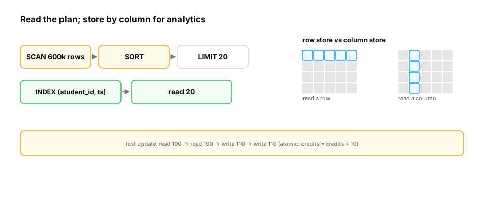
The incident. SELECT ... FROM progress WHERE student_id = ? ORDER BY ts DESC LIMIT 20 ran in 2 ms at launch and 1.8 s a year later. The plan showed a full scan of 40 million rows followed by a sort. A composite index on (student_id, ts) turned it back into a 1 ms lookup that reads only 20 rows.
You already know: B-trees, indexes, transactions and isolation levels in outline (Databases); Big-O and caches (Data structures, C++ memory).
1. Reading a query plan
The question. What does the database actually do with your query?
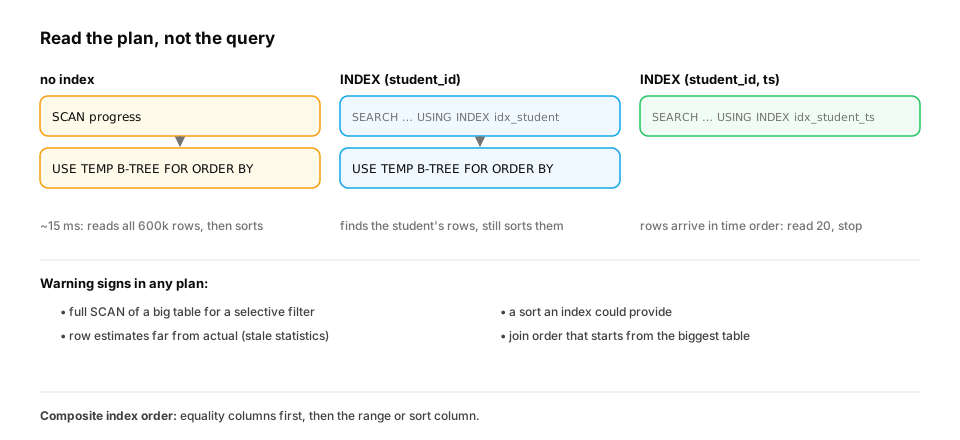
Start from nothing. The planner turns SQL into a plan: a tree of operators (scan a table or an index, filter, join with nested loops, hash or merge, sort, aggregate). It chooses among alternatives using statistics about table sizes and value distributions. EXPLAIN (or EXPLAIN QUERY PLAN in SQLite, EXPLAIN ANALYZE in PostgreSQL to also run it and show real timings) reveals the choice. The things to look for: full scans of big tables, sorts that an index could avoid, row estimates far from reality, and joins in an unexpected order.
import random, sqlite3, time

random.seed(0)
db = sqlite3.connect(":memory:")
db.execute("CREATE TABLE progress (student_id INT, lesson INT, ts INT, score REAL)")
db.executemany("INSERT INTO progress VALUES (?, ?, ?, ?)",
               ((random.randrange(50_000), random.randrange(500), t, random.random()) for t in range(600_000)))
q = "SELECT lesson, ts FROM progress WHERE student_id = 4242 ORDER BY ts DESC LIMIT 20"

def run(label):
    plan = [r[-1] for r in db.execute("EXPLAIN QUERY PLAN " + q)]
    t = time.perf_counter()
    for _ in range(20):
        db.execute(q).fetchall()
    print(f"{label:<28} {(time.perf_counter() - t) / 20 * 1000:7.2f} ms   plan: {plan}")

run("no index")
db.execute("CREATE INDEX idx_student ON progress(student_id)")
run("index on student_id")
db.execute("CREATE INDEX idx_student_ts ON progress(student_id, ts)")
run("index on (student_id, ts)")
Without an index, the database scans every row and sorts the matches. An index on student_id finds the student's rows directly but still sorts them; the composite index (student_id, ts) stores them already ordered by time, so the database reads the newest 20 entries and stops. Column order in a composite index matters: equality columns first, then the range or sort column.
In the run used to check this lesson, the three plans were SCAN progress plus USE TEMP B-TREE FOR ORDER BY (about 15 ms per query on 600,000 rows), then a SEARCH … USING INDEX idx_student that still sorts, and finally SEARCH … USING INDEX idx_student_ts with no sort step at all, under 0.01 ms.
In production. Teams don't read every plan. They find the expensive queries first, using PostgreSQL's
pg_stat_statementsextension (total time per normalized query), slow-query logs, or the warehouse's query history, and then runEXPLAIN (ANALYZE, BUFFERS)on the top few. A classic cause of a query that "suddenly got slow" with no code change is stale statistics: the planner still thinks a table has 10,000 rows when it has 40 million, and picks a plan that made sense for the small table. RunningANALYZE, or letting autovacuum keep up, refreshes them.
From production
A query's EXPLAIN ANALYZE shows 'estimated rows: 120, actual rows: 3,400,000' on a join input, and the planner chose a nested-loop join that takes minutes.
What's the most likely cause and first step?
Show the answer
B. The planner's statistics are badly out of date (or the predicate is hard to estimate); refresh statistics with ANALYZE, then re-check the plan before rewriting anything — A huge estimate-vs-actual gap means the planner is choosing blind. With fresh statistics it usually picks a hash join for millions of rows. Disabling join types globally hides the problem and hurts other queries.
2. When indexes help, and what they cost
The question. Why not index every column?
Start from nothing. Indexes speed up selective lookups (few matching rows), joins on the indexed key, and ORDER BY on indexed columns. They don't help when a query reads a large fraction of the table (a scan is cheaper than millions of index lookups), and they're defeated by wrapping the column in a function (WHERE date(ts) = ... can't use an index on ts; rewrite as a range). Every index costs storage and slows every INSERT and UPDATE, because it must be maintained. Add indexes for real query patterns, verified with the plan.
Here's that write cost, measured: the same 200,000 rows loaded into a table with 0, 2 and 5 indexes.
import random, sqlite3, time

random.seed(2)
rows = [(random.randrange(50_000), random.randrange(500), t, random.random()) for t in range(200_000)]

def load(n_indexes):
    db = sqlite3.connect(":memory:")
    db.execute("CREATE TABLE progress (student_id INT, lesson INT, ts INT, score REAL)")
    for cols in ["student_id", "lesson", "ts", "score", "student_id, ts"][:n_indexes]:
        db.execute(f"CREATE INDEX i_{len(cols)}_{cols[:3]} ON progress({cols})")
    t = time.perf_counter()
    db.executemany("INSERT INTO progress VALUES (?, ?, ?, ?)", rows)
    db.commit()
    return time.perf_counter() - t

base = load(0)
for k in (0, 2, 5):
    t = load(k)
    print(f"{k} indexes: {t * 1000:6.0f} ms to insert 200,000 rows ({t / base:.1f}x)")
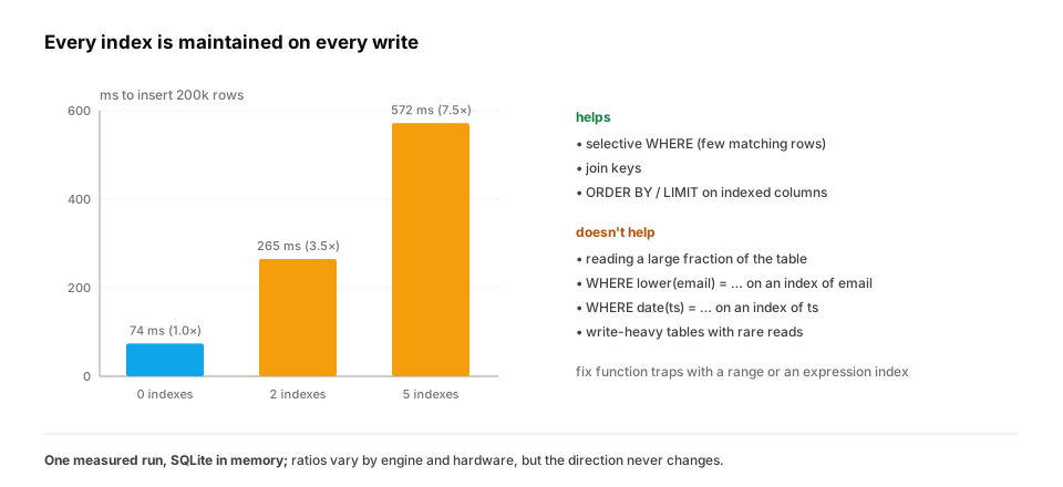
In the run used for this lesson, two indexes made the load about 3.5× slower and five about 7.5× slower (74, 265 and 572 ms). Exact timings vary by machine, but every index is another B-tree to update on every write. For a table that ingests events all day and is queried twice a week, most indexes cost more than they save.
In production. Ingestion pipelines often drop or defer secondary indexes during a large backfill and rebuild them afterwards, because building an index once over sorted data is much cheaper than maintaining it row by row. PostgreSQL can report unused indexes (
pg_stat_user_indexeswithidx_scan = 0), which are pure write overhead and safe candidates to drop after checking. Expression indexes such asCREATE INDEX ON users (lower(email))fix the function trap from the quiz below without changing the data.
Quick check
A query filters WHERE lower(email) = 'x@y.com' and an index exists on email. The plan shows a full scan. Why?
Show the answer
C. Applying a function to the column means the index on raw email values can't be used; store a normalized column or create an expression index on lower(email) — The index is ordered by email, not by lower(email). An expression (functional) index or a normalized column makes the predicate indexable.
3. Columnar engines: why analytics is fast in DuckDB and warehouses
The question. Why does SELECT AVG(score) FROM progress take seconds in the app database and milliseconds in a warehouse?
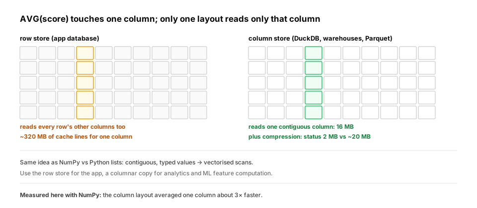
Start from nothing. Transactional databases store data by row (all columns of a row together), ideal for fetching or updating one record. Analytical engines (DuckDB, ClickHouse, BigQuery, Snowflake, Parquet files) store data by column: an aggregate over two columns reads only those two, the values of one column compress extremely well (similar values together), and operators run over vectors of values at a time (SIMD, cache-friendly). The same layout difference explains NumPy's speed over Python lists (Python internals). Use the transactional database for the app, and a columnar copy for analytics.
import time
import numpy as np

n, n_cols = 2_000_000, 20
rng = np.random.default_rng(0)
row_store = rng.random((n, n_cols))                     # row-major: each row's 20 columns are contiguous
col_store = np.asfortranarray(row_store)                # column-major: each column is contiguous

t = time.perf_counter(); r = row_store[:, 3].mean(); t_row = time.perf_counter() - t
t = time.perf_counter(); c = col_store[:, 3].mean(); t_col = time.perf_counter() - t
print(f"mean of one column: row layout {t_row * 1000:.1f} ms, column layout {t_col * 1000:.1f} ms ({t_row / t_col:.1f}x)")
print(f"bytes touched for that column: row layout ~{n * n_cols * 8 / 1e6:.0f} MB of cache lines, column layout {n * 8 / 1e6:.0f} MB")
codes = rng.integers(0, 5, n).astype(np.int8)           # e.g. 'status' with 5 values, dictionary-encoded
print(f"dictionary-encoded status column: {codes.nbytes / 1e6:.0f} MB instead of ~{n * 10 / 1e6:.0f} MB of strings")
Reading one column from the row layout strides over every row's other nineteen values, while the column layout reads one contiguous block. Columnar formats add compression (dictionary and run-length encoding) on top, which is why analytics engines read a fraction of the bytes.
In the checked run, the column layout averaged one column about 3× faster (5.9 ms vs 2.0 ms). The row layout drags about 320 MB of cache lines through the CPU for a 16 MB column, and dictionary-encoding a 5-value status column shrinks it to 2 MB from about 20 MB of strings.
In production. A common modern setup is the app's transactional database (PostgreSQL, MySQL) plus a columnar copy for analytics: a warehouse (BigQuery, Snowflake, Redshift), or Parquet files queried with DuckDB or Spark. Change-data-capture or nightly exports keep the copy fresh. ML training sets and feature tables almost always live on the columnar side, because training reads a few columns across many rows, which is exactly what columnar storage is built for.
From production
A data scientist runs SELECT user_id, AVG(session_minutes) FROM events GROUP BY user_id over two years of events directly on the production PostgreSQL primary. It takes 40 minutes and app latency spikes during the run.
What's the better setup?
Show the answer
A. Run analytics on a columnar copy (warehouse, or Parquet + DuckDB) fed by replication or exports, so scans read only the needed columns and don't compete with app traffic — Full-table aggregates are scans; an index won't make reading two years of rows cheap on a row store. A columnar copy reads just two columns, compressed, and isolates analytical load from the transactional workload.
4. Transactions, isolation and locks in practice
The question. Two requests update the same student's credits at once. What can go wrong?
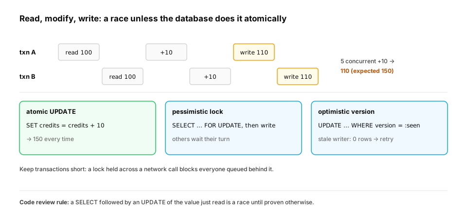
Start from nothing. A transaction groups statements so they commit atomically. Isolation levels decide what concurrent transactions see (Databases lesson): under the common default (read committed), a lost update happens when two transactions read the same value, each add to it, and the second write overwrites the first. Prevent it by updating atomically in one statement (SET credits = credits + 10), locking the row (SELECT ... FOR UPDATE), or using serializable isolation and retrying on conflict. Keep transactions short: locks held while waiting on a network call block everyone else.
import sqlite3, threading, time, os, tempfile

path = os.path.join(tempfile.mkdtemp(), "credits.db")
setup = sqlite3.connect(path); setup.execute("CREATE TABLE wallet (id INT PRIMARY KEY, credits INT)")
setup.execute("INSERT INTO wallet VALUES (1, 100)"); setup.commit(); setup.close()

def read_modify_write():
    con = sqlite3.connect(path, timeout=5, isolation_level=None)
    credits = con.execute("SELECT credits FROM wallet WHERE id = 1").fetchone()[0]   # read...
    time.sleep(0.05)                                                                   # ...app does something else...
    con.execute("UPDATE wallet SET credits = ? WHERE id = 1", (credits + 10,))         # ...write back a stale value
    con.close()

def atomic_update():
    con = sqlite3.connect(path, timeout=5, isolation_level=None)
    con.execute("UPDATE wallet SET credits = credits + 10 WHERE id = 1")
    con.close()

for name, fn in [("read-modify-write", read_modify_write), ("atomic UPDATE", atomic_update)]:
    con = sqlite3.connect(path); con.execute("UPDATE wallet SET credits = 100"); con.commit(); con.close()
    threads = [threading.Thread(target=fn) for _ in range(5)]
    [t.start() for t in threads]; [t.join() for t in threads]
    final = sqlite3.connect(path).execute("SELECT credits FROM wallet").fetchone()[0]
    print(f"{name:<18} 5 concurrent +10 updates -> {final} (expected 150)")
Five concurrent read-modify-write updates lose most of their increments, because each wrote back a value computed from a stale read; the single-statement atomic update gets every one. The same bug appears with any database and any language, and code review should catch the pattern.
In the checked run, the read-modify-write version ended at 110 instead of 150, so four of the five increments were lost. The atomic version ended at 150.
When you can't express the change as one statement: optimistic concurrency. Sometimes the new value comes from application logic: a plan change the user picked in one browser tab while another tab was still open. A version column turns "write back" into "write back only if nobody changed it since I read it":
import sqlite3, os, tempfile

path = os.path.join(tempfile.mkdtemp(), "plans.db")
con = sqlite3.connect(path, isolation_level=None)
con.execute("CREATE TABLE plans (user_id INT PRIMARY KEY, plan TEXT, version INT)")
con.execute("INSERT INTO plans VALUES (1, 'free', 1)")

def change_plan(new_plan, seen_version):
    """Optimistic concurrency: only write if nobody changed the row since we read it."""
    cur = con.execute("UPDATE plans SET plan = ?, version = version + 1 WHERE user_id = 1 AND version = ?",
                      (new_plan, seen_version))
    return cur.rowcount == 1

v = con.execute("SELECT version FROM plans WHERE user_id = 1").fetchone()[0]   # two tabs read version 1
print("tab A upgrades to pro:", change_plan("pro", v))
print("tab B downgrades to free with stale version:", change_plan("free", v))
print("final:", con.execute("SELECT plan, version FROM plans").fetchone())
Both tabs read version 1. Tab A's update matches and succeeds (True), bumping the row to version 2. Tab B's update still says WHERE version = 1, matches no row, and returns False. The application can then reload and ask the user, instead of silently overwriting the upgrade. The final row is ('pro', 2).
In production. ORMs support both styles: SQLAlchemy has a
version_id_coloption for optimistic versioning, and Django'sselect_for_update()takes a pessimistic row lock. HTTP APIs expose the same idea throughETagandIf-Matchheaders. It suits low-contention data such as user settings and documents. For hot counters like credits or inventory, the atomic single-statement update is simpler and never needs a retry.
From production
An inventory service runs stock = SELECT stock FROM items WHERE id = ? then, after checking stock > 0, UPDATE items SET stock = :stock - 1 WHERE id = ?. During a flash sale, 1,000 units are sold against 600 in stock.
What's the simplest correct fix?
Show the answer
C. A single atomic statement: UPDATE items SET stock = stock - 1 WHERE id = ? AND stock > 0, and treat 0 rows updated as 'sold out' — The check and the write must happen atomically. A conditional UPDATE does both in one statement: concurrent buyers can't both decrement the last unit, and rowcount tells you whether the purchase succeeded.
Check yourself
- What does EXPLAIN show, and what are three warning signs in a plan?
- Why does a composite index on
(student_id, ts)beat one onstudent_idalone for "latest 20 events"? - When doesn't an index help?
- Why are columnar engines fast for analytics?
- What causes a lost update, and name two ways to prevent it.
- What does an index cost, and how would you find indexes that aren't paying for themselves?
Answers
- The operator tree the planner chose. Full scans of big tables, sorts an index could avoid, row estimates far from reality, unexpected join orders.
- The composite index stores each student's rows already sorted by time, so the query reads the last 20 entries without sorting.
- Low selectivity (reading much of the table), functions applied to the column, and write-heavy tables where maintenance cost dominates.
- They read only the needed columns, compress similar values, and process vectors of values at a time.
- Two transactions read the same value and both write back modified copies. Atomic single-statement updates, row locks (SELECT FOR UPDATE), or serializable isolation with retries.
- Storage and slower writes, since every insert and update maintains it. Look for indexes the database reports as never used (e.g. idx_scan = 0 in PostgreSQL) and check them against real query patterns.
Exercise
Create a 300,000-row progress table and a query that counts completions per lesson in the last 30 days (WHERE ts >= ? then GROUP BY lesson). Measure it with no index, with an index on ts, and with a covering index on (ts, lesson), print each plan, and explain the result. Then rewrite a WHERE date(ts, 'unixepoch') >= '...' version and show that it can't use the index.
Solution
import random, sqlite3, time

random.seed(1)
db = sqlite3.connect(":memory:")
db.execute("CREATE TABLE progress (student_id INT, lesson INT, ts INT)")
start = 1_767_225_600                                                # 2026-01-01 in seconds
db.executemany("INSERT INTO progress VALUES (?, ?, ?)",
               ((random.randrange(50_000), random.randrange(500), start + random.randrange(365 * 86400)) for _ in range(300_000)))
cutoff = start + 335 * 86400
q = "SELECT lesson, COUNT(*) FROM progress WHERE ts >= ? GROUP BY lesson"
q_fn = "SELECT lesson, COUNT(*) FROM progress WHERE date(ts, 'unixepoch') >= '2026-12-02' GROUP BY lesson"

def measure(label, sql, args=()):
    plan = [r[-1] for r in db.execute("EXPLAIN QUERY PLAN " + sql, args)]
    t = time.perf_counter(); n = len(db.execute(sql, args).fetchall()); dt = (time.perf_counter() - t) * 1000
    print(f"{label:<30} {dt:7.1f} ms  groups={n}  plan={plan}")

measure("no index", q, (cutoff,))
db.execute("CREATE INDEX i_ts ON progress(ts)")
measure("index on ts", q, (cutoff,))
db.execute("CREATE INDEX i_ts_lesson ON progress(ts, lesson)")
measure("covering index (ts, lesson)", q, (cutoff,))
measure("function on ts (no index use)", q_fn)
The plain ts index finds the last month's rows (about 8% of the table), but then has to fetch each one from the table to read its lesson, one random lookup per row, which here is no faster than simply scanning everything. That's the selectivity lesson in action: an index pays off only when it avoids enough work. The covering index (ts, lesson) contains every column the query needs, so the database never touches the table and the query runs several times faster. Wrapping ts in date(...) throws that away: the plan becomes a SCAN of the whole index, because the index is ordered by raw ts, not by the function's output, and it's the slowest of the four. Rewrite such filters as ranges on the raw column.
This unlocks:
- SQL for ML — feature, experiment and vector queries that must run fast.
- SQL interview patterns and capstone — putting the track together.