The incident. A dashboard shows "average lesson rating: 4.6". A product manager asks why it fell to 3.9 when filtered to new students. Neither number is wrong; the first averaged ratings (heavily weighted towards a few prolific raters), the second averaged per-student averages. Aggregations answer exactly the question you write, which isn't always the one you meant.
You already know: SELECT, NULL and joins (previous lessons); means and distributions (D2).
1. GROUP BY and aggregate functions
The question. How do you turn many rows into one summary row per group?
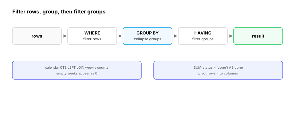
Start from nothing. GROUP BY partitions rows by the values of one or more columns; aggregates (COUNT, SUM, AVG, MIN, MAX) collapse each group to one value. Every selected column must be either grouped or aggregated. Aggregates ignore NULLs (except COUNT(*)), so COUNT(*), COUNT(col) and COUNT(DISTINCT col) answer three different questions, and AVG(col) silently averages only non-NULL values.
import sqlite3

db = sqlite3.connect(":memory:")
db.executescript("""
CREATE TABLE ratings (student_id INT, lesson TEXT, stars INT);
INSERT INTO ratings VALUES (1,'a',5),(1,'b',5),(1,'c',5),(1,'d',5),(1,'e',5),(2,'a',3),(3,'b',2),(3,'c',NULL),(4,'a',4);
""")
print(db.execute("SELECT COUNT(*), COUNT(stars), COUNT(DISTINCT student_id) FROM ratings").fetchone(),
      "<- rows, non-NULL ratings, distinct raters")
print("mean of all ratings:          ", round(db.execute("SELECT AVG(stars) FROM ratings").fetchone()[0], 2))
print("mean of per-student averages: ", round(db.execute(
    "SELECT AVG(avg_s) FROM (SELECT student_id, AVG(stars) AS avg_s FROM ratings GROUP BY student_id)").fetchone()[0], 2))
for row in db.execute("SELECT lesson, COUNT(stars) AS n, ROUND(AVG(stars), 2) FROM ratings GROUP BY lesson ORDER BY lesson"):
    print(row)
One enthusiastic student with five 5-star ratings pulls the per-rating mean to 4.25, while the average student rates 3.5. Decide which unit the question is about (ratings or students) and aggregate at that grain.
The same trap, one level up: Simpson's paradox. Averages also hide the mix of what was averaged. Here two models were evaluated on different mixes of easy and hard questions, a common accident when eval sets are sampled from different time periods or user groups:
import sqlite3

db = sqlite3.connect(":memory:")
db.execute("CREATE TABLE evals (model TEXT, difficulty TEXT, correct INT)")
def add(model, difficulty, n_correct, n_total):
    db.executemany("INSERT INTO evals VALUES (?, ?, ?)",
                   [(model, difficulty, 1)] * n_correct + [(model, difficulty, 0)] * (n_total - n_correct))
add("A", "easy", 81, 90);  add("A", "hard", 4, 10)      # model A was mostly tested on easy questions
add("B", "easy", 19, 20);  add("B", "hard", 36, 80)     # model B was mostly tested on hard ones

for row in db.execute("""SELECT model, difficulty, COUNT(*), ROUND(AVG(correct), 2)
                         FROM evals GROUP BY model, difficulty ORDER BY difficulty, model"""):
    print(row)
for row in db.execute("SELECT model, COUNT(*), ROUND(AVG(correct), 2) FROM evals GROUP BY model ORDER BY model"):
    print("overall", row)
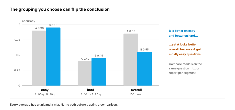
B beats A on easy questions (0.95 vs 0.9) and on hard ones (0.45 vs 0.4). Yet overall, A scores 0.85 and B only 0.55. A's overall average is mostly easy questions; B's is mostly hard ones. The overall number measures the question mix as much as the model.
In production. Model evaluation, A/B tests and fairness audits all hit this. The standard defences are to compare on the same evaluation set, to report per-segment results (difficulty, language, user tier) next to the overall number, and to check that the mix of segments is balanced between the arms of an experiment. When someone shows you a single average, ask "averaged over what, and in what mix?"
From production
A new support bot resolves 72% of tickets versus 80% for the old one, so the team plans a rollback. Then someone notices the new bot was rolled out first to enterprise customers, whose tickets are much harder.
What should the team do before deciding?
Show the answer
C. Compare resolution rates within each customer segment (or on the same ticket mix); the overall gap may be driven by the different mix, not the bot — If the new bot saw a harder mix, its overall rate can be lower even if it's better in every segment (Simpson's paradox). Segment-level comparisons, or a randomised split of the same traffic, separate the bot's effect from the mix.
2. WHERE vs HAVING
The question. How do you filter groups, as opposed to rows?
Start from nothing. WHERE filters rows before grouping; HAVING filters groups after aggregation, so it can use aggregates ("courses with at least 100 enrolments"). Filtering in WHERE when possible is both correct and cheaper (fewer rows reach the grouping step).
import sqlite3

db = sqlite3.connect(":memory:")
db.executescript("""
CREATE TABLE enrolments (student_id INT, course TEXT, status TEXT);
INSERT INTO enrolments VALUES (1,'ML101','done'),(2,'ML101','done'),(3,'ML101','dropped'),(4,'ML101','active'),
 (1,'SQL1','done'),(5,'SQL1','dropped'),(6,'LLM2','done'),(7,'LLM2','done'),(8,'LLM2','done');
""")
q = """
SELECT course, COUNT(*) AS enrolled,
       ROUND(AVG(CASE WHEN status = 'done' THEN 1.0 ELSE 0 END), 2) AS completion_rate
FROM enrolments
WHERE status != 'active'                -- rows: exclude students still in progress
GROUP BY course
HAVING COUNT(*) >= 3                    -- groups: only courses with enough finished outcomes
ORDER BY completion_rate DESC
"""
for row in db.execute(q):
    print(row)
The conditional average (AVG(CASE WHEN ... THEN 1.0 ELSE 0 END)) computes a rate in one pass, a pattern you'll use constantly. Excluding active enrolments in WHERE means the completion rate is over finished outcomes only, and HAVING drops courses with too few outcomes to trust.
The result has two rows: ('LLM2', 3, 1.0) and ('ML101', 3, 0.67). SQL1 had only two finished outcomes, so HAVING removed it.
A real-world refinement: don't let tiny groups win rankings. HAVING COUNT(*) >= n hides small groups entirely. Rankings such as "top-rated lessons" or "best prompts by thumbs-up rate" usually want to keep them, but discounted. A common approach is to add a few virtual ratings at the global average, so a group's score moves away from the average only as evidence accumulates:
import sqlite3

db = sqlite3.connect(":memory:")
db.execute("CREATE TABLE ratings (lesson TEXT, stars INT)")
data = {"intro-sql": [5], "joins": [5, 4, 5, 4, 4, 5, 4, 5, 5, 4] * 3, "ctes": [3, 4, 3, 4]}
for lesson, stars in data.items():
    db.executemany("INSERT INTO ratings VALUES (?, ?)", [(lesson, s) for s in stars])

q = """
WITH stats AS (SELECT lesson, COUNT(*) AS n, AVG(stars) AS mean FROM ratings GROUP BY lesson),
prior AS (SELECT AVG(stars) AS c FROM ratings)
SELECT lesson, n, ROUND(mean, 2) AS raw_mean,
       ROUND((n * mean + 10 * prior.c) / (n + 10), 2) AS smoothed     -- 10 'virtual' ratings at the global mean
FROM stats, prior
ORDER BY smoothed DESC"""
for row in db.execute(q):
    print(row)
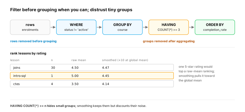
By raw mean, intro-sql (a single 5-star rating) would top the list at 5.0. Smoothed, it scores 4.45 and drops just below joins, which earned 4.47 from 30 ratings. A lesson with one review can't beat one with thirty consistent ones unless it really is better. The weight (10 here) controls how much evidence a group needs to pull away from the average.
In production. This is a simple form of Bayesian averaging, and variants are used wherever items with very different numbers of votes are ranked: product reviews, app stores, search results, and LLM leaderboards that report confidence intervals next to scores. In a feature pipeline, the same smoothing turns noisy per-user rates (click-through, completion) into features that don't swing wildly for new users.
Quick check
You want courses whose average rating is below 3. Where does the condition go?
Show the answer
B. HAVING AVG(stars) < 3 — The average exists only after grouping, so the filter must be in HAVING. WHERE runs before aggregation and can't reference aggregates.
3. Dates and buckets
The question. How do you count active students per week?
Start from nothing. Time series need buckets: truncate timestamps to day, week or month, then group. Decide and document the conventions: time zone (store UTC, convert for display), week start (Monday?), and whether empty buckets should appear as zeros (they won't unless you generate the calendar and left join). Numeric values bucket the same way: CAST(score / 10 AS INT) * 10 for score bands, or CASE for custom ranges.
import sqlite3

db = sqlite3.connect(":memory:")
db.execute("CREATE TABLE events (student_id INT, ts TEXT)")
rows = [(1, "2026-03-02 09:00"), (2, "2026-03-03 10:00"), (1, "2026-03-04 11:00"), (3, "2026-03-10 08:00"),
        (1, "2026-03-11 09:30"), (4, "2026-03-25 12:00"), (2, "2026-03-26 18:00")]
db.executemany("INSERT INTO events VALUES (?, ?)", rows)
q = """
WITH RECURSIVE weeks(week_start) AS (
    SELECT '2026-03-02' UNION ALL SELECT date(week_start, '+7 days') FROM weeks WHERE week_start < '2026-03-23'
),
activity AS (
    SELECT date(ts, '-6 days', 'weekday 1') AS week_start, COUNT(DISTINCT student_id) AS active
    FROM events GROUP BY 1
)
SELECT w.week_start, COALESCE(a.active, 0) AS weekly_active
FROM weeks w LEFT JOIN activity a USING (week_start)
ORDER BY w.week_start
"""
for row in db.execute(q):
    print(row)
The week of 16 March had no events; without the generated calendar it would simply be missing from the chart, and a line plot would quietly connect the neighbours as if nothing happened. (date(ts, '-6 days', 'weekday 1') is SQLite's way to find the Monday of a week: step back six days, then forward to the next Monday. The more obvious date(ts, 'weekday 1', '-7 days') sends events that happen on a Monday to the previous week, an off-by-one that deserves a unit test. Other databases use date_trunc('week', ts).)
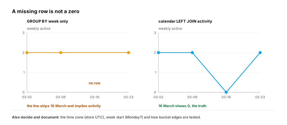
In production. Time zones cause the most expensive bucketing bugs. Store timestamps in UTC, and convert to the business's time zone before truncating to a day. Otherwise "daily revenue" for a company in India counts 05:30 to 05:30 local time, and a daylight-saving change makes one day 23 hours long. Warehouses provide calendar ("date spine") tables or generator functions, such as PostgreSQL's
generate_series, for the empty-bucket problem, and dbt projects often keep a shared date-spine model so every dashboard fills gaps the same way.
From production
A daily signups chart for a company in New York is built with GROUP BY date(created_at) on UTC timestamps. Marketing says signups from an 8 p.m. local-time campaign show up on the wrong day.
What's going on?
Show the answer
A. 8 p.m. in New York is already the next day in UTC, so date() on UTC timestamps assigns those signups to the following day; convert to the business time zone before truncating — Bucketing happens in whatever time zone the timestamp is in. Convert UTC to the reporting time zone first (e.g. AT TIME ZONE 'America/New_York' in PostgreSQL), then truncate, and document that choice on the chart.
4. Pivots
The question. How do you turn statuses (rows) into columns?
Start from nothing. A pivot turns values of one column into separate columns, using conditional aggregation: SUM(CASE WHEN status = 'done' THEN 1 ELSE 0 END) AS done. It's portable across databases (some also offer a PIVOT keyword) and is how most reporting tables are built.
import sqlite3

db = sqlite3.connect(":memory:")
db.executescript("""
CREATE TABLE enrolments (student_id INT, course TEXT, status TEXT);
INSERT INTO enrolments VALUES (1,'ML101','done'),(2,'ML101','done'),(3,'ML101','dropped'),(4,'ML101','active'),
 (1,'SQL1','done'),(5,'SQL1','dropped'),(6,'LLM2','done'),(7,'LLM2','active');
""")
q = """
SELECT course,
       SUM(status = 'active')  AS active,
       SUM(status = 'done')    AS done,
       SUM(status = 'dropped') AS dropped
FROM enrolments GROUP BY course ORDER BY course
"""
print(("course", "active", "done", "dropped"))
for row in db.execute(q):
    print(row)
Each course becomes one row with a count per status: ('LLM2', 1, 1, 0), ('ML101', 1, 2, 1) and ('SQL1', 0, 1, 1). In SQLite a comparison like status = 'done' evaluates to 1 or 0, so SUM counts the matches directly.
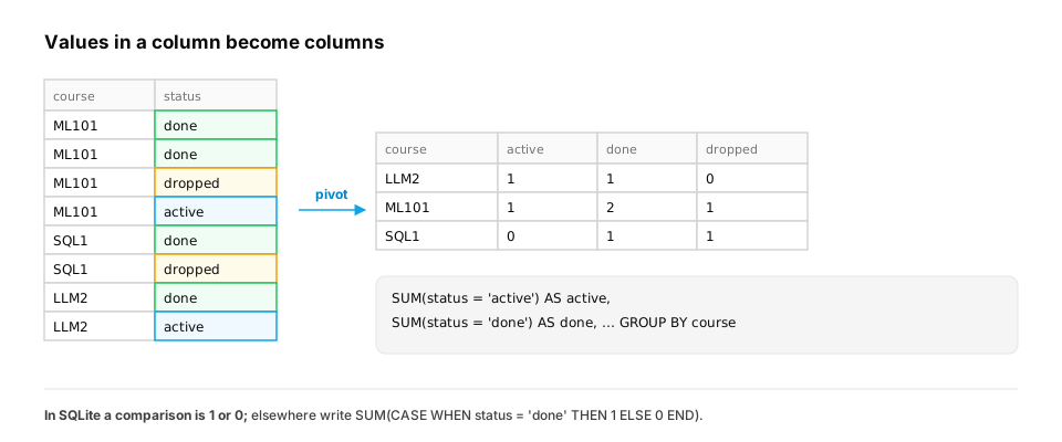
In production. Pivots are how event logs become ML features and reporting tables: one row per user with columns like
clicks_7d,purchases_7dandsupport_tickets_30d, each a conditional aggregate over the event table. The portableSUM(CASE WHEN … THEN 1 ELSE 0 END)form works everywhere. In PostgreSQL, comparisons are booleans, so writeCOUNT(*) FILTER (WHERE status = 'done')or the CASE form. One caution: a pivot's columns are fixed when the query is written, so a new status value silently goes uncounted. Pair pivots with a check that the statuses seen are the ones you expect.
From production
A pivot counts done, active and dropped per course. A new status paused is introduced in the product. The pivot's totals per course stop matching the enrolment counts.
Why, and what's a good safeguard?
Show the answer
C. The pivot's columns are fixed in the query, so 'paused' rows aren't counted anywhere; add an 'other' column (or a total) and alert when it's non-zero — Conditional aggregation only counts the values you named. An explicit SUM(status NOT IN (...)) AS other or a total column makes unexpected values visible instead of silently missing.
(In SQLite and PostgreSQL a boolean expression can be summed directly; in other databases write the explicit CASE.)
Check yourself
- What's the difference between
COUNT(*),COUNT(col)andCOUNT(DISTINCT col)? - Why can averaging ratings and averaging per-student averages disagree?
- When do you use WHERE versus HAVING?
- How do you make empty time buckets show up as zero?
- How can model B beat model A in every segment but lose overall?
- Why add "virtual" ratings at the global mean before ranking items by average rating?
Answers
- All rows; rows where col isn't NULL; distinct non-NULL values of col.
- Students with many ratings dominate the first; the second weights every student equally. They answer different questions.
- WHERE filters rows before grouping; HAVING filters groups using aggregates.
- Generate the full calendar (a recursive CTE or a date table) and left join the aggregates onto it with COALESCE(..., 0).
- If the two were evaluated on different mixes of segments (Simpson's paradox): the overall average reflects the mix as well as the model. Compare per segment or on the same mix.
- So items with very few ratings can't top the ranking on noise. Their score moves away from the average only as evidence accumulates.
Exercise
From an events(student_id, ts) table, compute for each week: weekly active students, new students (whose first-ever event is in that week), and returning students (active this week and also active in an earlier week). Use the data from section 3.
Solution
import sqlite3

db = sqlite3.connect(":memory:")
db.execute("CREATE TABLE events (student_id INT, ts TEXT)")
db.executemany("INSERT INTO events VALUES (?, ?)", [(1, "2026-03-02 09:00"), (2, "2026-03-03 10:00"), (1, "2026-03-04 11:00"),
    (3, "2026-03-10 08:00"), (1, "2026-03-11 09:30"), (4, "2026-03-25 12:00"), (2, "2026-03-26 18:00")])
q = """
WITH wk AS (SELECT DISTINCT student_id, date(ts, '-6 days', 'weekday 1') AS week FROM events),
first AS (SELECT student_id, MIN(week) AS first_week FROM wk GROUP BY student_id)
SELECT wk.week,
       COUNT(*) AS active,
       SUM(wk.week = first.first_week) AS new_students,
       SUM(wk.week > first.first_week) AS returning_students
FROM wk JOIN first USING (student_id)
GROUP BY wk.week ORDER BY wk.week
"""
for row in db.execute(q):
    print(row)
Reducing events to one row per student per week first (DISTINCT) fixes the grain, and comparing each week with the student's first week splits active students into new and returning. In the last week, Ben is returning (first seen three weeks earlier) and Dana is new.
This unlocks:
- Window functions — rankings and running totals without collapsing rows.
- CTEs and recursive queries — building multi-step queries like the calendar above.