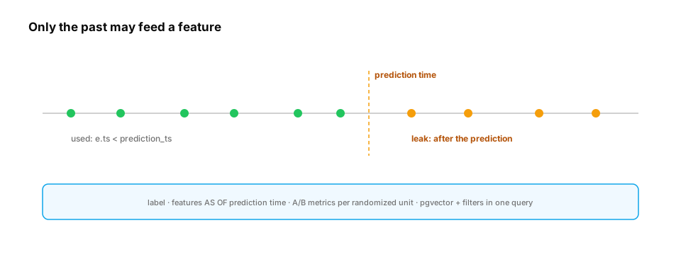
The incident. The dropout model's top feature was "lessons completed in total". For students in the training set, that count included lessons completed after the date the model was supposed to be predicting from, so students who stayed obviously had more lessons. In production, the feature only had the past, and the model's edge vanished.
You already know: window functions and CTEs (previous lessons); data leakage and feature stores (D3 Feature engineering); confidence intervals and A/B tests (D2); embeddings and vector search (D8).
1. Point-in-time correct training sets
The question. How do you build features that only use information available at prediction time?
Start from nothing. Each training example has a prediction time (the moment the model would have been asked) and a label from after it. Every feature must be computed from events strictly before that time: an as-of join. In SQL, join events to the label table with e.ts < l.prediction_ts (and often >= l.prediction_ts - window) and aggregate. Feature stores implement exactly this; writing it once by hand makes the failure mode unforgettable.
import random, sqlite3
import numpy as np

random.seed(0)
db = sqlite3.connect(":memory:")
db.execute("CREATE TABLE events (student INT, ts INT)")
db.execute("CREATE TABLE labels (student INT, prediction_ts INT, dropped INT)")
events, labels = [], []
for s in range(2000):
    engagement = random.random()
    dropped = int(random.random() < 0.6 - 0.4 * engagement)
    labels.append((s, 30, dropped))
    for day in range(60):
        active_after = day >= 30 and dropped
        if not active_after and random.random() < 0.1 + 0.3 * engagement:
            events.append((s, day))
db.executemany("INSERT INTO events VALUES (?, ?)", events)
db.executemany("INSERT INTO labels VALUES (?, ?, ?)", labels)

leaky = """SELECT l.dropped, COUNT(e.ts) FROM labels l LEFT JOIN events e ON e.student = l.student GROUP BY l.student"""
correct = """SELECT l.dropped, COUNT(e.ts) FROM labels l LEFT JOIN events e
             ON e.student = l.student AND e.ts < l.prediction_ts AND e.ts >= l.prediction_ts - 30 GROUP BY l.student"""

def auc(rows):
    y = np.array([r[0] for r in rows]); x = -np.array([r[1] for r in rows], float)   # fewer events -> more likely to drop
    pos, neg = x[y == 1], x[y == 0]
    return np.mean([(p > neg).mean() + 0.5 * (p == neg).mean() for p in pos])

print(f"AUC of 'event count' feature: leaky join {auc(db.execute(leaky).fetchall()):.2f}, point-in-time join {auc(db.execute(correct).fetchall()):.2f}")
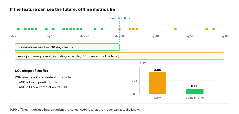
The leaky feature counts activity after day 30, which the label itself causes, so it predicts dropout almost perfectly offline; the point-in-time feature reflects what the model can actually know. Make the prediction timestamp an explicit column in every training table, and make every feature query take it as a parameter.
On these 2,000 simulated students, the same "event count" feature scores an AUC of 0.90 with the leaky join and 0.60 with the point-in-time join. The 0.90 is the number that would have shipped, and production would have delivered something close to 0.60.
In production. Feature stores exist largely to make this join impossible to get wrong. Feast's
get_historical_features, for example, takes an "entity dataframe" of IDs and event timestamps and performs a point-in-time join against each feature view. Two checks catch leakage before training: a feature with suspiciously high importance, and an offline metric far above anything the business has seen. When either happens, ask "could this feature have been known at prediction time?" before celebrating.
From production
A churn model's top feature is support_tickets_total, and offline AUC is 0.94. After launch, performance drops to roughly chance on that feature. The label is 'cancelled within 30 days after the snapshot date'.
What's the most likely cause?
Show the answer
D. Label leakage: the training feature counted tickets filed after the snapshot date, including the 'please cancel my account' tickets that the outcome itself generates; recompute it with e.ts < snapshot_ts — A feature that includes post-prediction events encodes the label. A point-in-time join (events strictly before the prediction timestamp, within a window) gives the model only what it will have in production.
2. Analysing an A/B test in SQL
The question. Did the new recommendation module increase lesson completion?
Start from nothing. Compute per-variant metrics at the unit of randomization (students, not events), then the difference and its confidence interval. SQL produces the sufficient statistics (counts, sums, sums of squares) and a few lines of arithmetic finish the job. Check the sample ratio first: if a 50/50 split produced 52/48, the assignment or logging is broken and the result isn't trustworthy (D10).
import math, random, sqlite3

random.seed(3)
db = sqlite3.connect(":memory:")
db.execute("CREATE TABLE assignment (student INT, variant TEXT)")
db.execute("CREATE TABLE completions (student INT, lesson INT)")
for s in range(20_000):
    v = "treatment" if random.random() < 0.5 else "control"
    db.execute("INSERT INTO assignment VALUES (?, ?)", (s, v))
    rate = 1.30 if v == "treatment" else 1.20
    for lesson in range(int(random.expovariate(1 / rate) + 0.5)):
        db.execute("INSERT INTO completions VALUES (?, ?)", (s, lesson))
q = """
WITH per_student AS (
    SELECT a.student, a.variant, COUNT(c.lesson) AS completed
    FROM assignment a LEFT JOIN completions c ON c.student = a.student GROUP BY a.student, a.variant
)
SELECT variant, COUNT(*), AVG(completed), SUM(completed * completed) FROM per_student GROUP BY variant ORDER BY variant
"""
stats = {}
for variant, n, mean, sumsq in db.execute(q):
    var = sumsq / n - mean ** 2
    stats[variant] = (n, mean, var)
    print(f"{variant:<10} n={n:>5}  mean completions {mean:.3f}")
(nc, mc, vc), (nt, mt, vt) = stats["control"], stats["treatment"]
diff, se = mt - mc, math.sqrt(vc / nc + vt / nt)
print(f"sample ratio {nt / (nt + nc):.3f} (expect 0.500)")
print(f"lift {diff:+.3f} completions per student ({diff / mc:+.1%}), 95% CI [{diff - 1.96 * se:+.3f}, {diff + 1.96 * se:+.3f}]")
The left join keeps students who completed nothing (zeros matter for the mean), aggregation at the student level respects the randomization unit, and the interval says whether the lift is distinguishable from zero. Doing this in SQL against the warehouse avoids exporting millions of rows.
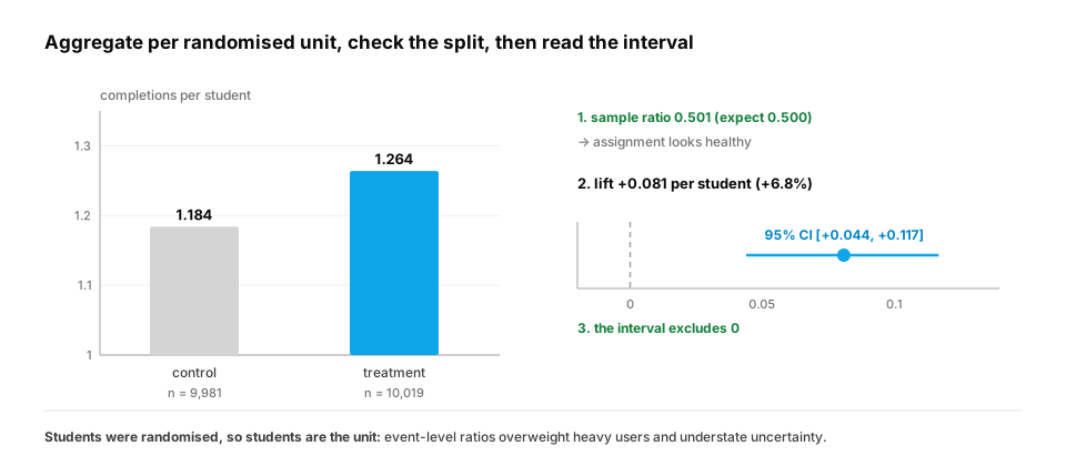
In this simulation, control averages 1.184 completions per student (n = 9,981) and treatment 1.264 (n = 10,019). The sample ratio is 0.501, healthy. The lift is +0.081 completions per student (+6.8%), with a 95% interval of [+0.044, +0.117], which excludes zero.
In production. Experimentation platforms compute exactly these per-unit sufficient statistics in the warehouse, often adding variance-reduction methods such as CUPED (which uses each user's pre-experiment metric to shrink the interval). The sample-ratio check is automated, because a mismatch usually means a logging or assignment bug, and no statistics can rescue a broken split. For LLM features, the same readout applies to online metrics like task completion and thumbs-up rate, with offline eval scores as a pre-launch gate (Evaluation path).
From production
An analyst computes an A/B test's completion rate as completed events / all events, per variant, by grouping the events table.
What's wrong?
Show the answer
D. The unit of analysis doesn't match the unit of randomization: heavy users contribute many events and their correlated behaviour makes the variance estimate wrong. Aggregate per student first, then compare student-level metrics — Students were randomized, so students are the independent units. Event-level analysis overweights heavy users and understates uncertainty, producing false positives.
3. Vector and hybrid search in Postgres
The question. Can Atlas keep embeddings next to the course data instead of a separate vector database?
Start from nothing. Yes, often. The pgvector extension adds a vector column type, distance operators (<-> L2, <=> cosine distance, <#> negative inner product) and approximate indexes (HNSW, IVFFlat; D8). The advantage is that filters and joins run in the same query, with the same permissions and transactions: "the 5 nearest chunks from the student's enrolled courses". Hybrid search combines a full-text rank (ts_rank over a tsvector) with vector similarity, for example by reciprocal rank fusion. A dedicated vector database earns its place at very large scale or with specialized needs.
-- schema and query in PostgreSQL with pgvector (not executed here)
CREATE EXTENSION IF NOT EXISTS vector;
CREATE TABLE chunks (
  id bigserial PRIMARY KEY, course_id int NOT NULL, body text NOT NULL,
  embedding vector(1024) NOT NULL, tsv tsvector GENERATED ALWAYS AS (to_tsvector('english', body)) STORED
);
CREATE INDEX ON chunks USING hnsw (embedding vector_cosine_ops);
CREATE INDEX ON chunks USING gin (tsv);
CREATE INDEX ON chunks (course_id);

-- hybrid search, permission-filtered, fused by reciprocal rank
WITH allowed AS (SELECT course_id FROM enrolments WHERE student_id = $1),
semantic AS (
  SELECT id, ROW_NUMBER() OVER (ORDER BY embedding <=> $2) AS r FROM chunks
  WHERE course_id IN (SELECT course_id FROM allowed) ORDER BY embedding <=> $2 LIMIT 50),
lexical AS (
  SELECT id, ROW_NUMBER() OVER (ORDER BY ts_rank(tsv, q) DESC) AS r
  FROM chunks, plainto_tsquery('english', $3) q
  WHERE tsv @@ q AND course_id IN (SELECT course_id FROM allowed) LIMIT 50)
SELECT c.id, c.body, COALESCE(1.0 / (60 + s.r), 0) + COALESCE(1.0 / (60 + l.r), 0) AS score
FROM chunks c LEFT JOIN semantic s USING (id) LEFT JOIN lexical l USING (id)
WHERE s.id IS NOT NULL OR l.id IS NOT NULL
ORDER BY score DESC LIMIT 10;
The permission filter sits inside both retrievals (D22 LLM platforms), and reciprocal rank fusion combines the two rankings without having to calibrate their scores against each other. The same logic can be prototyped in SQLite with plain tables and NumPy for the distances, which is how the exercise checks it.
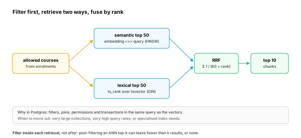
In production. The subtle failure is post-filtering. An approximate index returns, say, its 50 nearest neighbours first, and then a WHERE clause removes the ones the user may not see. If most of the nearest neighbours belong to other courses, the user gets 3 results, or none, while relevant allowed chunks sat just outside the top 50. Remedies include filtering inside the retrieval (as above), raising the candidate count for filtered queries, partitioning the index by tenant, or using a vector store with filter-aware search. Recent pgvector releases added iterative index scans for exactly this case. Whichever you choose, test filtered queries specifically: they're where retrieval quietly degrades.
From production
A multi-tenant RAG app runs SELECT … FROM chunks ORDER BY embedding <=> $q LIMIT 10 through an HNSW index and then drops chunks from other tenants in application code. Small tenants often get zero results.
What's happening, and what's a better design?
Show the answer
B. The ANN search returns the global top 10, mostly other tenants' chunks, and post-filtering removes them; filter by tenant inside the query (and/or partition the index per tenant, or raise the candidate count), so search happens within the allowed set — Approximate nearest-neighbour search plus a later filter can't recover candidates it never returned. Filtering inside the retrieval (or per-tenant indexes) keeps the top-k within what the user may see, which is also safer: unauthorised rows never leave the database.
Check yourself
- What is a point-in-time (as-of) join, and what goes wrong without it?
- Why compute A/B metrics per student, and why check the sample ratio?
- Why keep zero-activity students via a left join in an A/B analysis?
- What does pgvector add to Postgres, and when is it a good choice over a separate vector database?
- Why can post-filtering an approximate nearest-neighbour result return too few (or zero) results?
- A feature has suspiciously high importance and offline AUC is far above anything seen in production. What should you check first?
Answers
- Joining each example only to events before its prediction time. Without it, features include future information (often caused by the label), so offline metrics are inflated and production performance collapses.
- Students are the randomized, independent units; event-level analysis misweights users and understates variance. A sample-ratio mismatch signals broken assignment or logging.
- Students with no completions are part of the metric (zeros); an inner join would drop them and bias both means upwards.
- A vector type, distance operators and ANN indexes. When filters, joins, permissions and transactions with relational data matter and scale is moderate.
- The index returns its top-k over all rows; if most of those fail the filter, few or none remain, even though matching rows exist just outside the top-k. Filter inside the search instead.
- Leakage: whether the feature could have been known at prediction time, i.e. whether its query uses only events strictly before the prediction timestamp.
Exercise
Prototype the hybrid search from section 3 in SQLite + NumPy: store chunks with a course ID, body text and an embedding (as a BLOB), retrieve the top 5 by cosine similarity among chunks the student may see, the top 5 by a simple keyword-overlap score, and fuse them with reciprocal rank fusion (k = 60). Show that a chunk from a course the student isn't enrolled in never appears.
Solution
import sqlite3
import numpy as np

rng = np.random.default_rng(0)
db = sqlite3.connect(":memory:")
db.execute("CREATE TABLE chunks (id INTEGER PRIMARY KEY, course INT, body TEXT, emb BLOB)")
db.execute("CREATE TABLE enrolments (student INT, course INT)")
db.executemany("INSERT INTO enrolments VALUES (?, ?)", [(1, 10), (1, 11)])
bodies = ["gradient descent updates weights", "attention weighs tokens", "the kv cache stores keys and values",
          "backpropagation applies the chain rule", "dropout regularizes networks", "secret exam answers for course 12"]
courses = [10, 10, 11, 11, 10, 12]
topic = rng.standard_normal(16)
for i, (b, c) in enumerate(zip(bodies, courses)):
    e = rng.standard_normal(16) + (2.0 * topic if "kv" in b or "secret" in b else 0)
    db.execute("INSERT INTO chunks VALUES (?, ?, ?, ?)", (i, c, b, (e / np.linalg.norm(e)).astype(np.float32).tobytes()))

def hybrid(student, query_text, query_emb, k=60):
    rows = db.execute("""SELECT id, body, emb FROM chunks WHERE course IN
                         (SELECT course FROM enrolments WHERE student = ?)""", (student,)).fetchall()
    ids = [r[0] for r in rows]
    embs = np.stack([np.frombuffer(r[2], dtype=np.float32) for r in rows])
    sem = [ids[i] for i in np.argsort(-(embs @ query_emb))[:5]]
    q_words = set(query_text.split())
    lex = [r[0] for r in sorted(rows, key=lambda r: -len(q_words & set(r[1].split())))[:5] if q_words & set(r[1].split())]
    score = {}
    for ranking in (sem, lex):
        for rank, cid in enumerate(ranking, 1):
            score[cid] = score.get(cid, 0) + 1 / (k + rank)
    return sorted(score.items(), key=lambda kv: -kv[1])

q_emb = topic / np.linalg.norm(topic)
for cid, sc in hybrid(1, "what does the kv cache store", q_emb):
    body, course = db.execute("SELECT body, course FROM chunks WHERE id = ?", (cid,)).fetchone()
    print(f"{sc:.4f}  course {course}  {body}")
The KV-cache chunk ranks first because both retrievers agree on it. The "secret exam answers" chunk is similar to the query's embedding, but it belongs to course 12, where the student isn't enrolled, so the filter inside retrieval excludes it before ranking ever happens.
This unlocks:
- SQL interview patterns and capstone — the whole track in one analytics warehouse.