You already know: how memory layout decides speed — packed arrays beat scattered objects (Python internals §3, C++ §5).
Why this matters for Atlas. Thousands of students use Atlas at once. Each request must find that student's history (lookup), wait its turn fairly (scheduling), and fetch the best-matching lessons (ranking). Each of those jobs has a data structure built for it — and the same structures sit inside every LLM server you'll study later.
1. Big-O: how cost grows
The question. Two ways to find a student's record both take 1 ms with 100 students. Which one is still fast with 10 million?
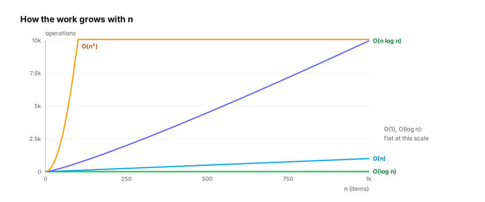
Start from nothing. Big-O describes how the work grows as the input size n grows, ignoring constant factors:
| Big-O | Meaning | n = 1,000 → n = 1,000,000 | Example |
|---|---|---|---|
| O(1) | same work regardless of n | 1 → 1 | dict lookup |
| O(log n) | +1 step each time n doubles | ~10 → ~20 | binary search, heap push |
| O(n) | work grows with n | 1k → 1M | scanning a list |
| O(n log n) | a bit more than linear | ~10k → ~20M | sorting |
| O(n²) | every pair | 1M → 10¹² | comparing all pairs |
Real-life analogy. Finding a word in a dictionary by opening near the right letter (log n) versus reading every page from the start (n).
Worked example.
import bisect, time

n = 1_000_000
ids = list(range(0, 2 * n, 2))          # sorted student ids
target = 1_999_998

id_set = set(ids)

t = time.perf_counter(); found = target in ids; scan = time.perf_counter() - t                 # O(n)
t = time.perf_counter(); i = bisect.bisect_left(ids, target); binary = time.perf_counter() - t  # O(log n)
t = time.perf_counter(); found_set = target in id_set; hashed = time.perf_counter() - t        # O(1)

print(f"scan {scan*1e3:.2f} ms | binary search {binary*1e6:.1f} µs | set lookup {hashed*1e6:.1f} µs")
The three timings differ by orders of magnitude: the scan takes milliseconds, while binary search and the set lookup take microseconds. Exact numbers depend on your machine.
Common trap. Big-O hides constants and memory layout. An O(n) scan of a packed NumPy array can beat an O(log n) walk through a pointer-heavy tree for small n.
How engineers spot complexity in practice: the doubling test. You rarely derive Big-O on paper for real code. Instead, run the code at size n and at 2n and compare. Linear work doubles, quadratic work roughly quadruples, and log-time work barely moves. Counting steps instead of timing gives a clean answer:
def dedupe_list(items):
    seen, steps = [], 0
    for x in items:
        steps += len(seen)              # `x in seen` may compare against every item kept so far
        if x not in seen:
            seen.append(x)
    return steps

def dedupe_set(items):
    seen, steps = set(), 0
    for x in items:
        steps += 1                      # one hash lookup
        seen.add(x)
    return steps

for n in (1_000, 2_000, 4_000):
    data = list(range(n))               # all unique: the worst case for the list version
    print(f"n={n:5}: list {dedupe_list(data):>10,} steps | set {dedupe_set(data):>6,} steps")
From 1,000 to 2,000 items, the list version goes from 499,500 to 1,999,000 steps (×4), then to 7,998,000 (×4 again). The set version goes 1,000 → 2,000 → 4,000 (×2 each time). A ×4 ratio per doubling is the fingerprint of O(n²). On real code you'd time it at a few sizes and look for the same pattern.
In production. Load tests and benchmarks at a single size miss this entirely. A job that takes 2 minutes on a 10% sample can take over 3 hours on the full data if it's quadratic (100× the work for 10× the data). Before a backfill or migration, run it at two sample sizes and check the ratio.
From production
A nightly feature job took 6 minutes on 1M rows. After the table grew to 2M rows, it takes 24 minutes.
What does that tell you?
Show the answer
A. Work roughly quadrupled when data doubled, so the job is likely O(n²): look for a membership check or lookup on a list inside a loop — Doubling n and seeing ×4 time is the signature of quadratic work. O(n) would be ~12 minutes, O(n log n) slightly more. Typical culprits are x in list, nested loops over rows, or repeated list.index.
2. Hash maps: jump straight to the answer
The question. How does Atlas find one student's session among millions without searching?
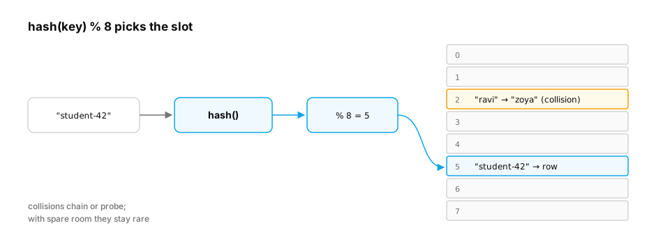
Start from nothing. A hash function turns a key (like "student-42") into a number. Take that number modulo the table size and you get a bucket index — the slot where the value lives. Lookup = compute hash → jump to slot: O(1) on average. Two keys can land in the same slot (a collision); the table handles it by probing the next slot or chaining, and it resizes when it gets too full so collisions stay rare.
Real-life analogy. A coat check: you hand over your coat, get ticket 57, and later they walk straight to hook 57.
Worked example — a tiny hash map, to see inside the box:
class TinyHashMap:
    def __init__(self, capacity=8):
        self.buckets = [[] for _ in range(capacity)]
        self.size = 0

    def _bucket(self, key):
        return self.buckets[hash(key) % len(self.buckets)]

    def put(self, key, value):
        bucket = self._bucket(key)
        for i, (k, _) in enumerate(bucket):
            if k == key:
                bucket[i] = (key, value)
                return
        bucket.append((key, value))
        self.size += 1
        if self.size > 0.75 * len(self.buckets):      # keep buckets short
            old = [kv for b in self.buckets for kv in b]
            self.buckets = [[] for _ in range(2 * len(self.buckets))]
            self.size = 0
            for k, v in old:
                self.put(k, v)

    def get(self, key, default=None):
        for k, v in self._bucket(key):
            if k == key:
                return v
        return default

sessions = TinyHashMap()
for i in range(100):
    sessions.put(f"student-{i}", {"lesson": i % 6})
print(sessions.get("student-42"), len(sessions.buckets))   # {'lesson': 0} 256
Where AI uses it. LLM servers cache attention data (the KV cache, D12) for prompts they've seen. Prefix caching hashes each block of prompt tokens so a repeated system prompt is found instantly instead of recomputed.
Common traps
- Mutable keys (
list) can't be hashed — their hash would change as they change. - Worst case is O(n) if many keys collide; real hash maps randomize hashes to make deliberate collisions hard.
The tiny map prints {'lesson': 0} 256. Inserting 100 keys with a 0.75 load limit doubled the table from 8 to 256 slots, five resizes in all. Each resize is O(n), but they get rarer as the table grows, so inserts stay O(1) on average (amortized), just like list.append.
From production
An inference server caches the KV data of prompt prefixes in a dict keyed by hash(tuple(token_ids)), and runs 8 worker processes behind a load balancer.
Within one worker, why is this lookup fast, and what should you watch for across workers?
Show the answer
C. It's O(1) on average because hashing jumps to a bucket. Each worker's cache is separate memory, so the same prompt can miss on another worker unless requests are routed to the worker that holds that prefix — Hash lookup is O(1) on average. But a dict lives in one process's memory, so a prefix cached on worker 3 is invisible to worker 5. Prefix-aware routing (D12) exists for exactly this reason. For anything shared or persisted, use a stable hash (hashlib), not hash().
3. Heaps and priority queues: always know who's next
The question. Requests arrive constantly. Atlas should answer paying users and short questions first, without re-sorting everything each time.
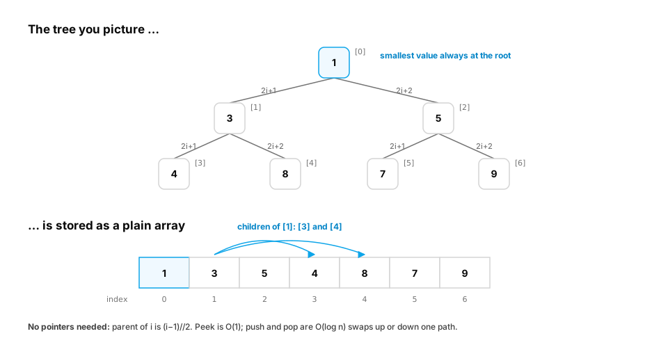
Start from nothing. A heap is a tree where every parent is smaller than its children (a min-heap), so the smallest item is always at the top. It's stored compactly in an array: the children of index i are at 2i+1 and 2i+2. Adding or removing an item only fixes one path from root to leaf: O(log n). Peeking at the top: O(1).
A priority queue is "a heap of (priority, item)" — exactly what a request scheduler needs.
Real-life analogy. An emergency room triage desk: the most urgent patient is always seen next, no matter when they arrived.
Worked example — scheduling requests, then top-K retrieval:
import heapq
import itertools

counter = itertools.count()          # tie-breaker keeps arrival order for equal priority
queue = []

def submit(priority, prompt):
    heapq.heappush(queue, (priority, next(counter), prompt))

submit(2, "free user: explain TCP")
submit(0, "pro user: debug my CUDA kernel")
submit(1, "pro user: quick definition of RAII")
submit(2, "free user: what is a heap?")

while queue:
    priority, _, prompt = heapq.heappop(queue)
    print(priority, prompt)

# Top-K: best 3 lesson scores out of a million in O(n log k), no full sort needed
import random
random.seed(0)
scores = [(random.random(), f"lesson-{i}") for i in range(1_000_000)]
print(heapq.nlargest(3, scores))
Where AI uses it. Inference servers (vLLM, TGI) keep waiting requests in priority queues; retrieval systems use top-K heaps to pick the best documents; beam search keeps the top-K partial sentences.
Common trap. Python's heapq is a min-heap. For "largest first", push negative priorities or use heapq.nlargest.
The scheduler serves priority 0 (the CUDA question) first, then priority 1, then the two free-user questions in arrival order. The counter breaks ties, so equal priorities never fall back to comparing the prompt strings. nlargest returns the three highest of a million scores without sorting the million.
A real-world example: top-K over a stream you can't store. Monitoring often needs "the slowest requests in the last hour" from a stream of millions of events, more than you want to keep in memory. A min-heap of size k solves it. It always holds the current top-k, and its smallest item, at the top, is the bar a new event must beat:
import heapq, random

random.seed(7)
stream = ((f"req-{i}", random.expovariate(1 / 120)) for i in range(1_000_000))   # latencies in ms

slowest = []                                  # min-heap of at most 3 (latency, id) pairs
for req_id, ms in stream:
    if len(slowest) < 3:
        heapq.heappush(slowest, (ms, req_id))
    elif ms > slowest[0][0]:                  # beats the smallest of the current top 3
        heapq.heapreplace(slowest, (ms, req_id))

for ms, req_id in sorted(slowest, reverse=True):
    print(f"{req_id}: {ms:,.0f} ms")
print("items held in memory:", len(slowest))
Out of a million simulated requests (mean 120 ms), the three slowest are req-311906 at 1,722 ms, req-658851 at 1,710 ms and req-663247 at 1,595 ms. The program never held more than 3 items. That's O(n log k) time and O(k) memory, the same pattern a vector database uses to keep the top-k nearest neighbours while it scans candidates (Vector databases).
Quick check
You must keep the 100 highest-scoring documents from a stream of 50 million scored documents, using as little memory as possible. Which approach fits?
Show the answer
D. A min-heap capped at 100: compare each new score with the heap's smallest and replace it if larger — A size-k min-heap keeps exactly the current top-k, and its root is the threshold to beat. That's O(n log k) time and O(k) memory. Sorting needs all 50M in memory and O(n log n) time.
4. Tries: share the beginning, save the work
The question. Many prompts start with the same system prompt. How can we recognise the shared beginning instantly?
Start from nothing. A trie (prefix tree) stores sequences character by character (or token by token) along branches. Sequences that share a prefix share the same path. Checking whether anything starts with "expl" means walking 4 steps — independent of how many items are stored.
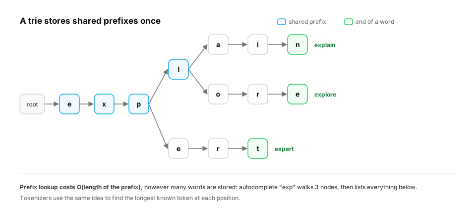
Real-life analogy. A building's directory: Floor 3 → Wing B → Room 12. People going to Wing B share the first two steps.
Worked example.
class Trie:
    def __init__(self):
        self.root = {}

    def insert(self, tokens):
        node = self.root
        for t in tokens:
            node = node.setdefault(t, {})
        node["<end>"] = True

    def longest_shared_prefix(self, tokens):
        node, depth = self.root, 0
        for t in tokens:
            if t not in node:
                break
            node, depth = node[t], depth + 1
        return depth

cache = Trie()
system = ["You", "are", "Atlas", ",", "a", "tutor", "."]
cache.insert(system + ["Explain", "TCP"])
cache.insert(system + ["Explain", "heaps"])

new_prompt = system + ["Explain", "RAII"]
reused = cache.longest_shared_prefix(new_prompt)
print(f"{reused} of {len(new_prompt)} tokens already computed")   # 8 of 9
Where AI uses it. Radix-tree prefix caching (SGLang's RadixAttention) reuses the KV cache of shared prompt prefixes; tokenizers and autocomplete use prefix trees too.
The example reports 8 of 9 tokens already computed: the 7-token system prompt plus "Explain" match a stored path, and only "RAII" is new. In a real server, a system prompt is often hundreds or thousands of tokens, and every request that shares it skips recomputing them. That's why prompt-caching features ask you to put stable content (instructions, tool definitions, documents) first and variable content last. A change near the start breaks the shared path for everything after it.
From production
A team adds the current timestamp at the very top of their 2,000-token system prompt 'so the model knows the date'. Prefix-cache hit rate drops to almost zero and latency rises.
Why?
Show the answer
C. The trie/prefix match breaks at the first differing token; a changing first line makes every request's prefix unique, so nothing after it can be reused — Prefix reuse follows a shared path from the start. Put stable content first and variable content (dates, user input) after it, so the long stable prefix stays shared.
5. Graphs: steps that depend on each other
The question. An agent must fetch a lesson, then generate a quiz and a summary from it, then email both. What order is valid, and what can run in parallel?
Start from nothing. A graph is nodes (things) connected by edges (relationships). If edges have a direction and no cycles, it's a DAG (directed acyclic graph) — the standard shape of workflows and data pipelines. A topological sort lists nodes so every dependency comes before what needs it. Nodes whose dependencies are all done can run at the same time.
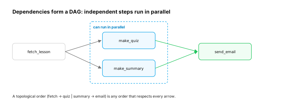
Real-life analogy. Cooking dinner: you can chop vegetables and boil water at the same time, but you can't serve until both are done.
Worked example.
from graphlib import TopologicalSorter

# node: set of nodes it depends on
workflow = {
    "make_quiz": {"fetch_lesson"},
    "make_summary": {"fetch_lesson"},
    "send_email": {"make_quiz", "make_summary"},
}
ts = TopologicalSorter(workflow)
ts.prepare()
step = 1
while ts.is_active():
    ready = list(ts.get_ready())          # everything runnable right now
    print(f"step {step}: run in parallel -> {sorted(ready)}")
    ts.done(*ready)
    step += 1
Where AI uses it. Agent frameworks (LangGraph and similar) model agents as graphs of steps; ML pipelines (Airflow, Kubeflow) are DAGs; neural networks themselves are computation graphs that autograd walks backwards (D2, D4).
Common trap. Cycles. A cycle in a "workflow" means it can never finish; TopologicalSorter raises CycleError — agent loops need an explicit stop condition instead.
The workflow runs in three steps: ['fetch_lesson'], then ['make_quiz', 'make_summary'] together, then ['send_email']. If the two middle steps are LLM calls taking 3 seconds each, running them in parallel saves 3 seconds on every request. Here is the trap, caught before anything runs:
from graphlib import TopologicalSorter, CycleError

agent = {
    "plan": {"reflect"},          # plan waits for reflect...
    "act": {"plan"},
    "reflect": {"act"},           # ...which waits for act, which waits for plan
}
try:
    list(TopologicalSorter(agent).static_order())
except CycleError as e:
    print("CycleError:", e.args[1])
It prints the cycle it found: ['plan', 'act', 'reflect', 'plan']. Agents really do loop (plan → act → reflect → plan…), but as a bounded loop with a stop condition (max steps, a "done" signal, a budget), not as a dependency graph that can never be satisfied.
From production
A pipeline has steps load → (clean, embed) → index → evaluate, where clean and embed both depend only on load, and index needs both.
With unlimited workers, what is the minimum number of sequential rounds?
Show the answer
D. 4: load; clean and embed together; index; evaluate — Topological 'levels' give the rounds: {load}, {clean, embed}, {index}, {evaluate}. Steps in the same level have all their dependencies done and can run in parallel.
6. Trees for search: B-trees and decision trees
The question. Hash maps answer "find exactly this key". How do we answer "find all students who joined between March and May"?
Start from nothing. A balanced search tree keeps keys sorted, so range queries walk a contiguous slice. Databases use B-trees: very wide trees where each node holds hundreds of keys and fills one disk page, so even a billion keys need only 3–4 node reads. (You'll see this again in Databases.) A different kind of tree — a decision tree — asks yes/no questions to classify data (D3).
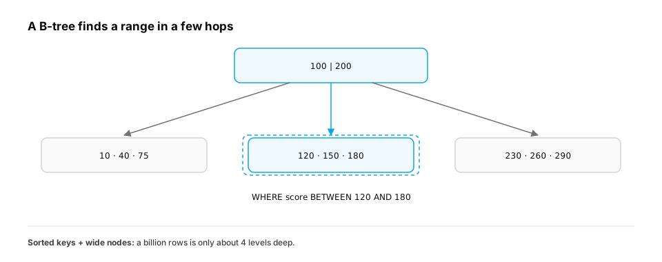
Worked example — sorted keys support range queries; hashing doesn't:
import bisect

join_days = sorted([3, 15, 40, 62, 75, 90, 120, 150])   # days since launch
lo, hi = 60, 100
start, end = bisect.bisect_left(join_days, lo), bisect.bisect_right(join_days, hi)
print(join_days[start:end])     # [62, 75, 90]
| Need | Structure | Cost |
|---|---|---|
| Exact lookup by key | Hash map | O(1) average |
| Next most important | Heap | O(log n) push/pop |
| Shared prefixes | Trie | O(length of key) |
| Dependencies / order | DAG + topological sort | O(nodes + edges) |
| Range queries, sorted order | B-tree / sorted array | O(log n + results) |
From production
A deduplication job checks each of 5 million documents against a growing list of seen hashes.
What change fixes its quadratic running time?
Show the answer
B. Store seen hashes in a hash set so each membership check is O(1) on average — List membership is O(n), making the job O(n²); a hash set makes it O(n) overall.
Check yourself
- Recall: Why is a Python
dictlookup O(1) on average but not guaranteed? - Apply: You need the 10 most relevant of 5 million documents. Sort everything, or use a heap?
- Predict: In the trie example, how many tokens could be reused for
system + ["Summarise", "TCP"]? - Diagnose: A job's runtime goes from 10 minutes to 40 when its input doubles. What complexity does that suggest, and what would you look for?
- Design: Why should stable content go at the start of a prompt when the server uses prefix caching?
Answers
- Collisions: if many keys hash to the same bucket, lookups scan that bucket. Resizing and randomized hashing keep that rare.
- A heap of size 10 (
heapq.nlargest): O(n log 10) instead of O(n log n). - 7 — the shared system prompt; "Summarise" doesn't match "Explain".
- ×4 for ×2 input suggests O(n²). Look for list membership checks,
index()or nested loops over the data inside a loop. - Prefix matching follows the tokens from the start and stops at the first difference. Stable content first keeps a long shared prefix that every request can reuse.
Exercise
Build RequestScheduler with submit(user_tier, prompt) and next_batch(k) that returns up to k prompts, pro users first, and within a tier the oldest first. Add an "aging" rule so a free user who has waited more than 5 submissions moves up one tier.
Solution
import heapq
import itertools

class RequestScheduler:
    TIERS = {"pro": 0, "free": 1}

    def __init__(self, age_limit=5):
        self.heap, self.clock, self.age_limit = [], itertools.count(), age_limit

    def submit(self, tier, prompt):
        heapq.heappush(self.heap, [self.TIERS[tier], next(self.clock), prompt])

    def _age(self):
        now = next(self.clock)
        for entry in self.heap:
            if entry[0] > 0 and now - entry[1] > self.age_limit:
                entry[0] -= 1
        heapq.heapify(self.heap)

    def next_batch(self, k):
        self._age()
        return [heapq.heappop(self.heap)[2] for _ in range(min(k, len(self.heap)))]

s = RequestScheduler()
s.submit("free", "old free question")
for i in range(6):
    s.submit("pro", f"pro question {i}")
print(s.next_batch(3))   # ['old free question', 'pro question 0', 'pro question 1']
                         # it waited too long, was promoted to pro, and is the oldest there
This unlocks:
- Operating systems — page tables are lookup tables; schedulers are priority queues.
- D12 KV cache & batching — prefix caching (hash maps, tries) and request scheduling (heaps).
- D8 Vector databases — top-K search over embeddings.
- D9 Agent architectures — agents as graphs.
Sources: Python docs — heapq, graphlib, bisect, "Dictionaries" time complexity; Cormen et al., Introduction to Algorithms (heaps, B-trees); vLLM docs — "Automatic Prefix Caching"; Zheng et al., SGLang (2024), RadixAttention.