You already know: the gradient points uphill and backprop computes it for every weight (Calculus §2, §4); cross-entropy is the loss models minimize (Probability §5).
Why this matters for Atlas. Gradients only say which way is downhill at this exact spot. How big a step to take, how to use the last few steps, and when to slow down decide whether training takes an hour, takes a week, or never works. Every model in this course is trained with the optimizers on this page.
1. Gradient descent and the learning rate
The question. We know the downhill direction. How far should we step?
Start from nothing. Gradient descent repeats one rule:
w ← w − η · ∇L(w)
where η (eta) is the learning rate. Too small: training crawls. Too large: each step overshoots the valley and the loss bounces or explodes. The best value depends on how curved the loss is, which is why the learning rate is the single most important hyperparameter.
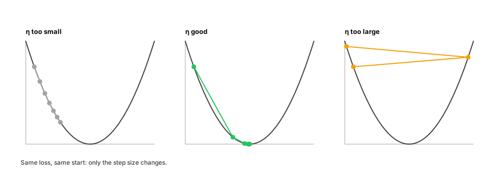
Real-life analogy. Walking down a dark hill: tiny steps are safe but slow; giant leaps jump past the bottom onto the other side.
Worked example.
def train(lr, steps=20):
    w = 0.0                                   # minimize L(w) = (w - 3)^2
    for _ in range(steps):
        w -= lr * 2 * (w - 3)
    return w, (w - 3) ** 2

for lr in [0.01, 0.1, 0.5, 0.9, 1.1]:
    w, loss = train(lr)
    print(f"lr={lr:<4}: w={w:9.3f}  loss={loss:.3g}")
For this bowl, any learning rate above 1.0 diverges: each step multiplies the distance to the minimum by |1 − 2η|, which exceeds 1 when η > 1.
From production
A training loss goes down for the first 200 steps, then oscillates with growing amplitude and finally becomes NaN.
What's the first thing to try?
Show the answer
A. Lower the learning rate (or add warmup and gradient clipping): steps larger than the curvature allows overshoot and then diverge — Growing oscillation is the signature of a step size beyond the stable limit (about 2/λ along the sharpest direction). Lowering the learning rate, warming up, or clipping gradient norms restores stability.
2. Stochastic and mini-batch gradient descent
The question. The training set has a billion examples. Do we really compute the gradient over all of them for every single step?
Start from nothing. The full-data gradient is an average over examples. A small random mini-batch (say 32–4,096 examples) gives a noisy but unbiased estimate of that average (Probability §3: standard error shrinks like 1/√batch). So we take many cheap, slightly noisy steps instead of few expensive exact ones — stochastic gradient descent (SGD). The noise even helps escape poor flat regions.
One pass through the whole dataset is an epoch.
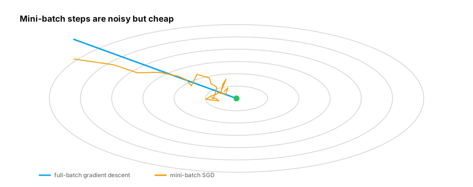
Worked example — fitting a line with mini-batches:
import numpy as np

rng = np.random.default_rng(0)
X = rng.uniform(0, 10, 10_000)
y = 2.5 * X + 1.0 + rng.normal(0, 1.0, X.size)       # true slope 2.5, intercept 1.0

w, b, lr, batch = 0.0, 0.0, 0.01, 64
for epoch in range(5):
    order = rng.permutation(X.size)
    for start in range(0, X.size, batch):
        idx = order[start:start + batch]
        err = (w * X[idx] + b) - y[idx]
        w -= lr * 2 * (err * X[idx]).mean()          # gradient of mean squared error
        b -= lr * 2 * err.mean()
    mse = ((w * X + b - y) ** 2).mean()
    print(f"epoch {epoch + 1}: w={w:.3f} b={b:.3f} mse={mse:.3f}")
Common trap. Not shuffling: if data is sorted (all cats, then all dogs), each batch pulls the model in one direction.
Quick check
Why do practitioners often scale the learning rate up when they increase the batch size?
Show the answer
C. A larger batch gives a less noisy gradient estimate (noise shrinks like 1/√B), so larger steps stay stable; rules like linear scaling with warmup work up to a point, after which returns diminish — The mini-batch gradient is an average, so its noise falls as the batch grows. Less noise permits bigger steps, but beyond a 'critical batch size' extra samples add little information per step.
3. Momentum: remember where you were going
The question. In a long narrow valley, plain SGD zig-zags across the walls and barely moves along the floor. How do we fix that?
Start from nothing. Keep a running average of past gradients — a velocity — and step along it:
v ← β·v + ∇L · w ← w − η·v (β ≈ 0.9)
Directions that keep agreeing (along the valley floor) build up speed; directions that flip sign every step (across the walls) cancel out.
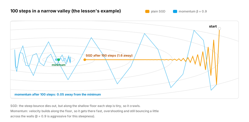
Real-life analogy. A heavy ball rolling downhill: it doesn't stop at every bump, and its weight carries it in the consistent direction.
Worked example.
import numpy as np

def loss_grad(w):                    # narrow valley: steep in w[1], shallow in w[0]
    return np.array([0.02 * w[0], 2.0 * w[1]])

def run(beta, lr=0.9, steps=100):
    w, v = np.array([10.0, 1.0]), np.zeros(2)
    for _ in range(steps):
        v = beta * v + loss_grad(w)
        w = w - lr * v
    return np.linalg.norm(w)

print(f"plain SGD distance to minimum: {run(beta=0.0):.3f}")
print(f"momentum  distance to minimum: {run(beta=0.9):.3f}")
From production
Plain SGD on a problem with very different curvature along two directions zig-zags across the narrow direction and crawls along the long one.
What does momentum change?
Show the answer
D. It averages recent gradients, so oscillating components cancel across steps while the consistent direction accumulates speed — Momentum keeps a running sum (velocity) of gradients. Back-and-forth components cancel out; the steady downhill component adds up, so progress along the valley floor speeds up.
4. Adam and AdamW: a step size per weight
The question. Some weights get huge gradients, others tiny ones. Can each weight get its own step size?
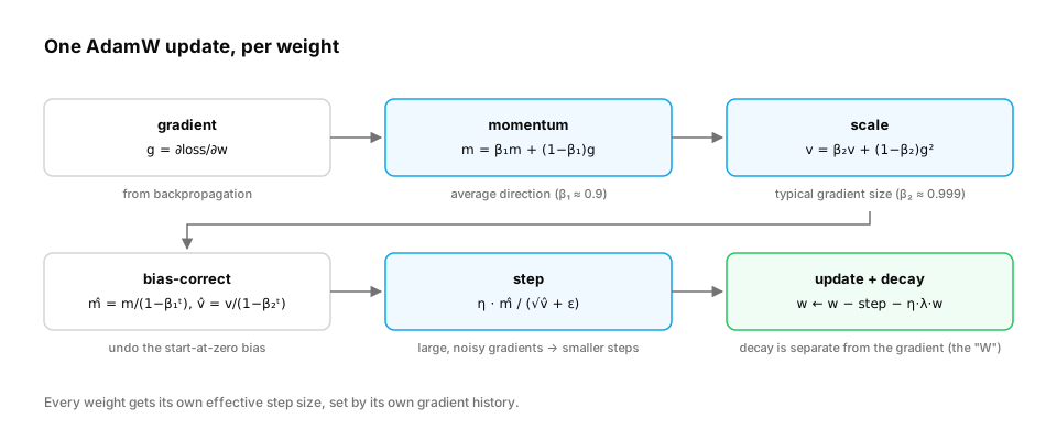
Start from nothing. Adam keeps two running averages per weight:
m— the average gradient (momentum),v— the average squared gradient (how large gradients usually are).
The step is η · m̂ / (√v̂ + ε): weights with consistently large gradients take smaller relative steps, and rarely-updated weights take larger ones. (m̂, v̂ correct a bias toward zero in early steps.)
AdamW fixes how weight decay (shrinking weights to prevent overfitting) interacts with Adam: it applies decay directly to the weights, separately from the gradient-based step. AdamW is the default optimizer for training transformers and LLMs.
Worked example — Adam from scratch vs plain SGD on badly scaled features:
import numpy as np

rng = np.random.default_rng(1)
X = np.column_stack([rng.normal(0, 1, 2000), rng.normal(0, 100, 2000)])   # features on very different scales
y = X @ np.array([3.0, 0.05]) + rng.normal(0, 0.1, 2000)

def grad(w):
    return 2 * X.T @ (X @ w - y) / len(y)

def sgd(lr=1e-5, steps=500):
    w = np.zeros(2)
    for _ in range(steps):
        w -= lr * grad(w)
    return w

def adamw(lr=0.05, steps=500, b1=0.9, b2=0.999, eps=1e-8, weight_decay=0.0):
    w, m, v = np.zeros(2), np.zeros(2), np.zeros(2)
    for t in range(1, steps + 1):
        g = grad(w)
        m = b1 * m + (1 - b1) * g
        v = b2 * v + (1 - b2) * g ** 2
        m_hat, v_hat = m / (1 - b1 ** t), v / (1 - b2 ** t)
        w -= lr * m_hat / (np.sqrt(v_hat) + eps) + lr * weight_decay * w
    return w

print("true  :", [3.0, 0.05])
print("SGD   :", sgd().round(3))      # [0.03 0.049]: the weight on the small-scale feature barely moves
print("AdamW :", adamw().round(3))
SGD needs a learning rate small enough for the large-scale feature, which leaves the other one almost untouched. Adam adapts per weight.
Common traps
- Reusing an SGD learning rate with Adam (typical Adam rates are much smaller, e.g. 1e-4 to 3e-4 for transformers).
- Applying weight decay to everything — biases and normalization weights are usually excluded.
From production
Fine-tuning with Adam(weight_decay=0.01) and with AdamW(weight_decay=0.01) gives noticeably different results, and the team assumed they were the same thing.
What's the difference?
Show the answer
B. Adam's weight_decay adds the decay to the gradient, so it gets rescaled by the adaptive denominator and weights with large gradient history are barely regularised; AdamW applies decay directly to the weights, decoupled from the adaptive step — Loshchilov & Hutter (2019) showed L2-in-the-gradient interacts badly with Adam's per-weight scaling. Decoupled weight decay (AdamW) shrinks every weight at the intended rate and is the default for transformer training.
5. Learning-rate schedules: warmup and decay
The question. Why do LLM training runs change the learning rate over time?
Start from nothing. Early in training, Adam's statistics are unreliable and gradients can be wild, so we warm up: ramp the learning rate from ~0 to its peak over the first few hundred or thousand steps. Later, smaller steps let the model settle into a good minimum, so we decay — most commonly a cosine curve down to a small fraction of the peak.
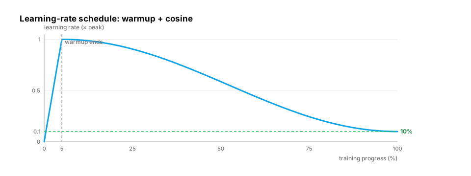
Worked example.
import math

def lr_at(step, total=10_000, peak=3e-4, warmup=500, floor_ratio=0.1):
    if step < warmup:
        return peak * (step + 1) / warmup
    progress = (step - warmup) / (total - warmup)
    floor = peak * floor_ratio
    return floor + (peak - floor) * 0.5 * (1 + math.cos(math.pi * progress))

for s in [0, 250, 499, 500, 2500, 5000, 7500, 9999]:
    print(f"step {s:>5}: lr = {lr_at(s):.2e}")
In production / interviews. A loss curve that suddenly spikes and doesn't recover often means the learning rate is too high for that stage. Typical responses: lower the peak, lengthen warmup, add gradient clipping (Calculus §5), or resume from a checkpoint before the spike. Interview question: "Why use warmup with Adam?"
Quick check
Why do large language model training runs usually start with a learning-rate warmup?
Show the answer
C. Early on, Adam's second-moment estimates are unreliable and the loss surface can be sharp, so full-size steps can blow up; ramping the learning rate up over the first steps keeps updates stable — At initialisation, adaptive denominators are based on very few samples, and curvature can be high. A short linear warmup avoids early divergence. Cosine or linear decay later helps settle into a good minimum.
6. The landscape: local minima, saddle points and flat regions
The question. Won't gradient descent get stuck in a bad local minimum?
Start from nothing. In very high dimensions, true bad local minima turn out to be rarer than early researchers feared. More common obstacles are saddle points (downhill in some directions, uphill in others) and plateaus (nearly flat regions). Noise from mini-batches, momentum and adaptive steps all help move through them. Wide, flat minima also tend to generalize better than sharp ones.
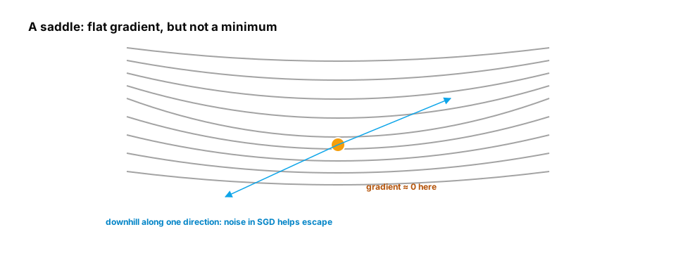
Worked example — a saddle point traps exact gradient descent but not noisy descent:
import numpy as np

def grad(w):                     # f(x, y) = x^2 - y^2 + y^4 / 4  (saddle at the origin, minima at y = ±√2)
    x, y = w
    return np.array([2 * x, -2 * y + y ** 3])

def descend(noise, steps=300, lr=0.05, seed=0):
    rng = np.random.default_rng(seed)
    w = np.array([1.0, 0.0])                 # start exactly on the saddle's ridge
    for _ in range(steps):
        w = w - lr * (grad(w) + noise * rng.normal(size=2))
    return w.round(3)

print("exact gradients:", descend(noise=0.0))   # stuck at the saddle (0, 0)
print("noisy gradients:", descend(noise=0.1))   # escapes to a minimum near y = ±1.414
Quick check
Training loss spikes and diverges in the first few hundred steps with AdamW, but trains well later in previous runs. What's the standard fix?
Show the answer
A. Use learning-rate warmup (start small and ramp up) so early updates, made with poorly estimated second moments, stay small — Adam's second-moment estimates are noisy at the start; warmup prevents oversized early steps.
Check yourself
- Recall: What two running averages does Adam keep per weight?
- Apply: Your loss decreases very slowly and smoothly. Change the learning rate up or down?
- Predict: In section 1, what happens with
lr = 1.0exactly? - Diagnose: Loss falls, then oscillates with growing amplitude and becomes NaN. What happened and what do you change?
- Recall: How does AdamW's weight decay differ from Adam with L2 regularisation?
Answers
- The mean of gradients (
m) and the mean of squared gradients (v). - Up (cautiously) — slow, smooth progress usually means steps are too small.
|1 − 2·1| = 1: the distance never shrinks —wbounces between 0 and 6 forever.- The step size exceeded the stable limit for the sharpest direction. Lower the learning rate, add warmup, or clip gradients.
- AdamW shrinks weights directly, decoupled from the adaptive step; Adam with L2 adds decay to the gradient, where the per-weight scaling distorts it.
Exercise
Implement a tiny training loop for 2-class logistic regression with mini-batch AdamW, cosine schedule with warmup, and gradient clipping at norm 1.0. Train on two Gaussian blobs and report accuracy per epoch.
Solution
import math
import numpy as np

rng = np.random.default_rng(0)
n = 2000
X = np.vstack([rng.normal([-1, -1], 1, (n // 2, 2)), rng.normal([1.5, 1.5], 1, (n // 2, 2))])
y = np.r_[np.zeros(n // 2), np.ones(n // 2)]
Xb = np.column_stack([X, np.ones(n)])                       # add a bias column

def lr_at(step, total, peak=0.05, warmup=50):
    if step < warmup:
        return peak * (step + 1) / warmup
    return peak * 0.5 * (1 + math.cos(math.pi * (step - warmup) / (total - warmup)))

w, m, v = np.zeros(3), np.zeros(3), np.zeros(3)
epochs, batch = 5, 64
total = epochs * math.ceil(n / batch)
step = 0
for epoch in range(epochs):
    for idx in np.array_split(rng.permutation(n), math.ceil(n / batch)):
        p = 1 / (1 + np.exp(-Xb[idx] @ w))
        g = Xb[idx].T @ (p - y[idx]) / len(idx)              # gradient of cross-entropy
        g *= min(1.0, 1.0 / (np.linalg.norm(g) + 1e-12))     # clip to norm 1
        step += 1
        m = 0.9 * m + 0.1 * g
        v = 0.999 * v + 0.001 * g ** 2
        lr = lr_at(step - 1, total)
        w -= lr * (m / (1 - 0.9 ** step)) / (np.sqrt(v / (1 - 0.999 ** step)) + 1e-8) + lr * 0.01 * w
    acc = ((Xb @ w > 0) == y).mean()
    print(f"epoch {epoch + 1}: accuracy {acc:.3f}")
This unlocks:
- Information theory — what exactly the cross-entropy loss is measuring.
- D3 Supervised learning — linear and logistic regression trained exactly like this.
- D5 LLM pretraining — AdamW, warmup and cosine decay at scale.
- D15 Training memory optimization — Adam's
mandvdouble the memory per weight.
Sources: Kingma & Ba, Adam (2015); Loshchilov & Hutter, Decoupled Weight Decay Regularization (AdamW, 2019) and SGDR (cosine schedules, 2017); Goodfellow et al., Deep Learning ch. 8; Dauphin et al., Identifying and attacking the saddle point problem (2014).