You already know: vectors and the softmax function (Linear algebra §5); gradients tell us how to reduce an error (Calculus §2).
Why this matters for Atlas. An LLM never "knows" the next word — it outputs a probability distribution over every possible next token and samples from it. And when we change Atlas, we can't just eyeball a few answers: we need statistics to tell real improvement from luck.
1. Probability distributions
The question. What does a model actually output before it "chooses" a word?
Start from nothing. A probability is a number between 0 and 1 describing how likely something is. A distribution assigns probabilities to every possible outcome, and they add up to 1.
| Distribution | Outcomes | AI example |
|---|---|---|
| Bernoulli | yes / no with probability p | "Is this answer correct?" |
| Categorical | one of K options | Next token from a 50,000-token vocabulary |
| Normal (Gaussian) | any real number, bell-shaped around a mean μ with spread σ | Weight initialization, measurement noise |
A model's raw scores (logits) become a categorical distribution through softmax: pᵢ = e^{zᵢ} / Σⱼ e^{zⱼ} — exponentiate (all positive), then divide by the total (sums to 1).
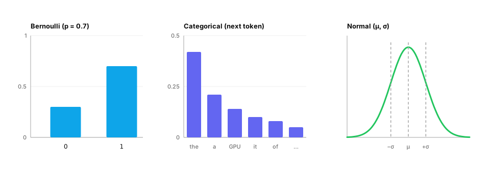
Real-life analogy. A weather forecast: "70% rain" is a Bernoulli distribution; "40% sun, 35% cloud, 25% rain" is categorical.
Worked example.
import numpy as np

vocab = ["memory", "paging", "pizza", "pages", "the"]
logits = np.array([2.1, 3.0, -1.0, 2.6, 0.5])        # raw model scores

probs = np.exp(logits - logits.max())
probs /= probs.sum()
for word, p in sorted(zip(vocab, probs), key=lambda t: -t[1]):
    print(f"{word:7s} {p:.3f}")
print("sum:", probs.sum())                             # 1.0
Common trap. "The model is 60% confident, so it's right 60% of the time." Only if the model is calibrated — modern LLMs often aren't, which D10 measures.
From production
A classifier outputs scores (2.1, 0.3, −1.0) for three intents, and a downstream rule says 'act only if the top intent has probability > 0.9'.
What must happen to the scores before that rule makes sense?
Show the answer
A. Convert them to a distribution (softmax gives non-negative values summing to 1), and ideally check calibration, since a raw score or an uncalibrated softmax isn't a reliable confidence — Thresholds on 'probability' need actual probabilities. Softmax turns logits into a distribution, but modern networks are often over-confident, so teams calibrate (e.g. temperature scaling on a validation set) before trusting thresholds.
2. Conditional probability and Bayes' rule
The question. A hallucination detector flags 95% of real hallucinations. It flagged this answer. How likely is it really a hallucination?
Start from nothing. P(A | B) — "probability of A given B" — restricts attention to cases where B happened. Bayes' rule flips a conditional around:
P(H | flag) = P(flag | H) · P(H) / P(flag)
The often-forgotten piece is P(H), the base rate: how common hallucinations are in the first place.
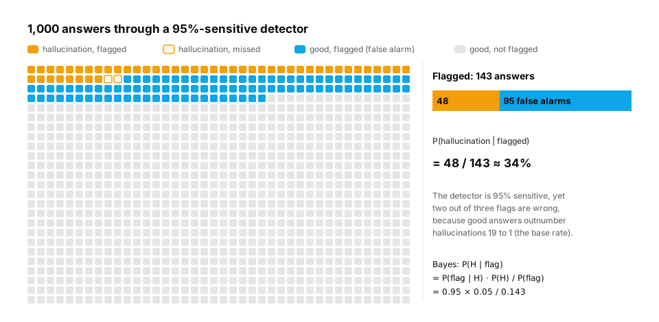
Worked example — counting beats formulas:
answers = 1000
base_rate = 0.05          # 5% of answers hallucinate
sensitivity = 0.95        # detector catches 95% of hallucinations
false_positive = 0.10     # and wrongly flags 10% of good answers

bad = answers * base_rate
good = answers - bad
flagged_bad = bad * sensitivity
flagged_good = good * false_positive
p = flagged_bad / (flagged_bad + flagged_good)
print(f"flagged: {flagged_bad:.0f} real + {flagged_good:.0f} false alarms")
print(f"P(hallucination | flagged) = {p:.2f}")       # 0.33 — not 0.95!
Real-life analogy. A medical test for a rare disease: even an accurate test produces mostly false alarms when the disease is rare.
In production / interviews. This is why guardrail precision drops in real traffic, and why you report precision and recall (D3, D10), not just "95% accurate". Interview question: "Our safety classifier is 99% accurate, yet most of its blocks are wrong. How?"
From production
A toxicity filter catches 99% of toxic messages and wrongly flags 2% of normal ones. Only 0.5% of messages are toxic.
Roughly what share of flagged messages are actually toxic?
Show the answer
C. About 20%: of 10,000 messages, ~50 are toxic and ~49.5 get flagged, while ~199 of the 9,950 normal ones are falsely flagged, so 49.5 / 248.5 ≈ 0.2 — Bayes' rule with a low base rate: even an accurate detector produces mostly false alarms when the condition is rare. This is why moderation queues need human review or a second-stage model.
3. Expectation, variance and the law of large numbers
The question. Each Atlas answer costs a different number of tokens. What should we budget per answer, and how wrong could that budget be?
Start from nothing.
- Expected value
E[X] = Σ xᵢ pᵢ— the long-run average outcome. - Variance
Var[X] = E[(X − E[X])²]— how spread out outcomes are; the standard deviation σ is its square root, in the original units. - Law of large numbers — the average of many independent samples approaches
E[X]. - Standard error — the uncertainty of a sample average shrinks like
σ / √n. Four times as many samples halves the uncertainty.
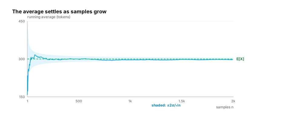
Worked example.
import numpy as np

rng = np.random.default_rng(42)
tokens = rng.lognormal(mean=5.0, sigma=0.6, size=100_000)   # skewed, like real answer lengths

print(f"expected tokens ≈ {tokens.mean():.0f}, std ≈ {tokens.std():.0f}")
for n in [10, 100, 1000, 10000]:
    sample = rng.choice(tokens, size=n, replace=False)
    se = sample.std(ddof=1) / np.sqrt(n)
    print(f"n={n:>5}: mean {sample.mean():6.1f} ± {1.96 * se:5.1f}  (95% interval)")
Common trap. Budgeting for the mean when the distribution is skewed: long answers dominate cost and latency. Look at percentiles (p50, p95, p99) — inference SLAs (D12) are written in p95/p99.
From production
Average tokens per answer is 400, but the standard deviation is 600 and a few answers run to 8,000 tokens.
What should a cost budget for 1 million answers be based on, and what else should you plan for?
Show the answer
D. The mean (≈ 400M tokens total, by the law of large numbers the total is predictable), while per-request limits and latency SLOs must plan for the heavy tail: cap max_tokens and watch p99 — Totals over many requests concentrate around n·mean, so budgets use the mean. Individual requests don't: the tail drives timeouts, context overflows and worst-case latency, so limits and alerts target percentiles.
4. Sampling: temperature, top-k and top-p
The question. Why does the same prompt give different answers, and how do we control that?
Start from nothing. Generating text = repeatedly sampling a token from the model's distribution. Three common controls reshape the distribution first:
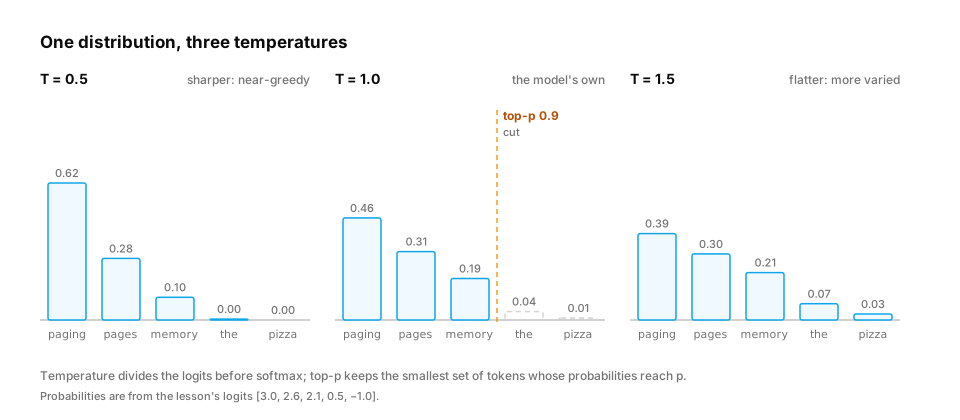
- Temperature T — divide logits by T before softmax. T < 1 sharpens (more predictable); T > 1 flattens (more varied). T → 0 approaches greedy decoding (always the top token).
- Top-k — keep only the k most likely tokens, renormalize.
- Top-p (nucleus) — keep the smallest set of tokens whose probabilities add up to at least p, renormalize.
Worked example.
import numpy as np

rng = np.random.default_rng(0)
vocab = np.array(["paging", "pages", "memory", "the", "pizza"])
logits = np.array([3.0, 2.6, 2.1, 0.5, -1.0])

def distribution(logits, temperature=1.0, top_k=None, top_p=None):
    z = logits / temperature
    p = np.exp(z - z.max()); p /= p.sum()
    order = np.argsort(-p)
    keep = np.ones_like(p, dtype=bool)
    if top_k is not None:
        keep[order[top_k:]] = False
    if top_p is not None:
        cumulative = np.cumsum(p[order])
        cutoff = np.searchsorted(cumulative, top_p) + 1      # smallest set reaching top_p
        keep[order[cutoff:]] = False
    p = np.where(keep, p, 0.0)
    return p / p.sum()

for settings in [dict(temperature=0.5), dict(temperature=1.5), dict(top_k=2), dict(top_p=0.9)]:
    p = distribution(logits, **settings)
    samples = rng.choice(vocab, size=1000, p=p)
    counts = {w: int((samples == w).sum()) for w in vocab if (samples == w).any()}
    print(settings, counts)
In production. Use low temperature (or greedy) for extraction, classification and code; higher for brainstorming. For evaluation, fix the seed and settings, or sample several times and report variance.
Quick check
top-p (nucleus) sampling with p = 0.9 is applied to a next-token distribution. What does it do?
Show the answer
B. Samples from the smallest set of most-likely tokens whose total probability reaches 0.9, after renormalising, so the long tail of unlikely tokens is never sampled — Nucleus sampling adapts the candidate set to the distribution: a confident distribution yields a small nucleus, an uncertain one a larger set. It removes tail tokens that cause incoherent output while keeping diversity.
5. Maximum likelihood: where the training loss comes from
The question. Why are almost all classifiers and LLMs trained with "cross-entropy loss"?
Start from nothing. Given data, the best parameters are those that make the observed data most probable — maximum likelihood. For independent examples, the probability of all of them is the product ∏ p(yᵢ). Products of many small numbers underflow, and products are awkward to differentiate, so we take the log (turning products into sums) and negate it to get something to minimize:
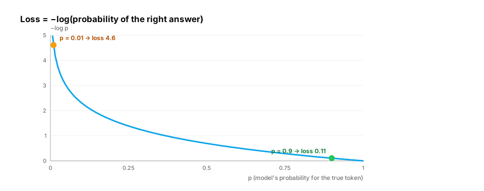
loss = −(1/N) Σ log p_model(correct answerᵢ) — the negative log-likelihood, also called cross-entropy loss.
If the model gives the correct next token probability 0.9, the loss contribution is −log 0.9 = 0.105; at 0.01 it's 4.6. Confident wrong answers are punished hard.
Worked example — estimating a coin's bias by maximum likelihood:
import numpy as np

flips = np.array([1, 1, 0, 1, 1, 0, 1, 1, 1, 0])      # 7 heads out of 10
candidates = np.linspace(0.01, 0.99, 99)
nll = [-(flips * np.log(p) + (1 - flips) * np.log(1 - p)).sum() for p in candidates]
best = candidates[int(np.argmin(nll))]
print(f"maximum-likelihood p = {best:.2f}")          # 0.70 = 7/10

print([round(-np.log(p), 3) for p in (0.9, 0.5, 0.1, 0.01)])   # [0.105, 0.693, 2.303, 4.605]
This is the bridge to information theory (lesson 5): cross-entropy measures how many "bits of surprise" the model suffers on real data.
From production
A model trained with cross-entropy assigns probability 0.0 to a correct token in one validation example.
What happens to the cross-entropy loss, and why does training try hard to avoid it?
Show the answer
C. The loss is −log 0 = ∞: maximum likelihood punishes confident mistakes without limit, which is why models keep small probabilities on alternatives (and why label smoothing exists) — Cross-entropy is the negative log-likelihood. A probability of 0 for an observed outcome makes the likelihood 0 and the loss infinite. In practice, frameworks clamp or work in log space, and label smoothing discourages extreme confidence.
6. Did the new model really improve? Confidence intervals and A/B tests
The question. Atlas v2 scores 82% on 200 test questions; v1 scored 78%. Ship it?
Start from nothing. Scores on a finite test set are estimates with noise. Questions to ask:
- Confidence interval — a range likely to contain the true score. For an accuracy p̂ on n items:
p̂ ± 1.96 · √(p̂(1 − p̂)/n)(95%, normal approximation). - Paired comparison — both models answered the same questions, so compare per question. That removes the variation from question difficulty.
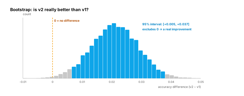
- Bootstrap — resample the test set with replacement thousands of times and recompute the difference; the spread of those differences is its uncertainty. No formulas needed.
- p-value — the probability of seeing a difference at least this large if there were truly no difference. Small p-values suggest a real effect; they don't measure how big or how important it is.
Worked example.
import numpy as np

rng = np.random.default_rng(7)
n = 200
v1 = np.zeros(n, dtype=bool); v1[:156] = True     # v1 right on 156/200 = 78%
v2 = v1.copy()
v2[156:170] = True                                # v2 fixes 14 questions v1 got wrong...
v2[:6] = False                                    # ...and breaks 6 that v1 got right -> 164/200 = 82%
order = rng.permutation(n); v1, v2 = v1[order], v2[order]

def ci(acc, n):
    half = 1.96 * np.sqrt(acc * (1 - acc) / n)
    return acc - half, acc + half

print(f"v1 {v1.mean():.3f}  95% CI {np.round(ci(v1.mean(), n), 3)}")
print(f"v2 {v2.mean():.3f}  95% CI {np.round(ci(v2.mean(), n), 3)}")

diffs = []
for _ in range(10_000):
    idx = rng.integers(0, n, n)                   # resample questions, keep pairs together
    diffs.append(v2[idx].mean() - v1[idx].mean())
lo, hi = np.percentile(diffs, [2.5, 97.5])
print(f"paired bootstrap difference: {v2.mean() - v1.mean():+.3f}, 95% CI [{lo:+.3f}, {hi:+.3f}]")
print("significant" if lo > 0 or hi < 0 else "not distinguishable from zero with 200 questions")
Output: v1 0.780, v2 0.820, difference +0.040 with a 95% interval of about [−0.005, +0.085]. The interval still includes zero, so 200 questions can't prove v2 is better — even though it "won" by 4 points. Either collect more questions or treat it as a tie.
Common traps
- Testing many variants and shipping the luckiest (the multiple comparisons problem). Hold out a fresh test set for the final decision.
- Peeking at an A/B test daily and stopping as soon as it "looks significant" inflates false positives.
- Statistically significant ≠ important: a +0.3% gain may not justify 2× cost.
In production / interviews. Interview question: "How many evaluation questions do you need to detect a 2-point accuracy improvement?" (The standard error shrinks as 1/√n; to resolve ±1 point at 80% accuracy you need roughly 1.96² × 0.8 × 0.2 / 0.01² ≈ 6,000 questions — paired comparisons need fewer.)
From production
A new model scores 81.0% vs the old model's 80.2% on a 500-question eval.
What's the right conclusion?
Show the answer
C. The difference is well within the ±3–4 point confidence interval for 500 questions; it's not evidence of improvement without a larger or paired analysis — The standard error of an accuracy near 80% on 500 items is about 1.8 points, so a 0.8-point gap is noise.
Check yourself
- Recall: What does softmax guarantee about its outputs?
- Apply: You want deterministic, extraction-style answers. Temperature high or low?
- Predict: The base rate of hallucination falls from 5% to 1% with the same detector. Does
P(hallucination | flagged)go up or down? - Apply: Why do cost budgets use the mean tokens per answer while latency alerts use p99?
- Recall: What does top-p sampling keep, and why does it adapt to the model's confidence?
Answers
- Every output is positive and they sum to 1 — a valid probability distribution.
- Low (or greedy decoding).
- Down — with fewer real hallucinations, a larger share of flags are false alarms (about 9% in that case).
- Totals over many requests concentrate around n × mean (law of large numbers), but individual requests don't: the heavy tail drives timeouts and worst-case latency.
- The smallest set of most-likely tokens whose probabilities add up to p. A confident distribution gives a small set; an uncertain one gives a larger set.
Exercise
Write compare_models(correct_a, correct_b, n_boot=10000) that takes two boolean arrays (same questions) and returns the accuracy difference, a 95% paired-bootstrap confidence interval, and a verdict ("A better", "B better", "inconclusive"). Then use it to answer: with these settings, how many questions are needed before a true 3-point gap is detected at least 80% of the time? (Simulate.)
Solution
import numpy as np

def compare_models(a, b, n_boot=2000, rng=None):
    rng = rng or np.random.default_rng(0)
    n = len(a)
    idx = rng.integers(0, n, (n_boot, n))
    diffs = b[idx].mean(axis=1) - a[idx].mean(axis=1)
    lo, hi = np.percentile(diffs, [2.5, 97.5])
    verdict = "B better" if lo > 0 else "A better" if hi < 0 else "inconclusive"
    return b.mean() - a.mean(), (lo, hi), verdict

rng = np.random.default_rng(1)
for n in [200, 800, 2000]:
    detected = 0
    for trial in range(100):
        a = rng.random(n) < 0.78
        b = np.where(rng.random(n) < 0.7, a, rng.random(n) < 0.88)   # true gap ≈ +3 points
        detected += compare_models(a, b, rng=rng)[2] == "B better"
    print(f"n={n:>4}: detected the improvement in {detected}% of simulated evaluations")
This unlocks:
- Optimization — minimizing the cross-entropy loss from section 5.
- Information theory — entropy, cross-entropy and KL divergence in bits.
- D3 ML evaluation and D10 LLM evaluation — precision/recall, calibration and significance in practice.
- D12 Inference — sampling strategies and p95/p99 latency.
Sources: Blitzstein & Hwang, Introduction to Probability; Efron & Tibshirani, An Introduction to the Bootstrap; Holtzman et al., The Curious Case of Neural Text Degeneration (2020, nucleus sampling); Miller, Adding Error Bars to Evals (Anthropic, 2024).