You already know: a model layer is a matrix multiplication y = W x + b (Linear algebra §3), and similarity can be scored with dot products (§2).
Why this matters for Atlas. Atlas's lesson-ranking formula has weights. Some rankings get good feedback, some bad. We need a precise answer to: "if I nudge this weight up a little, does the error go up or down, and by how much?" That number is a derivative, and computing it for millions of weights at once is backpropagation — the engine of all deep learning.
1. The derivative: how fast does the output change?
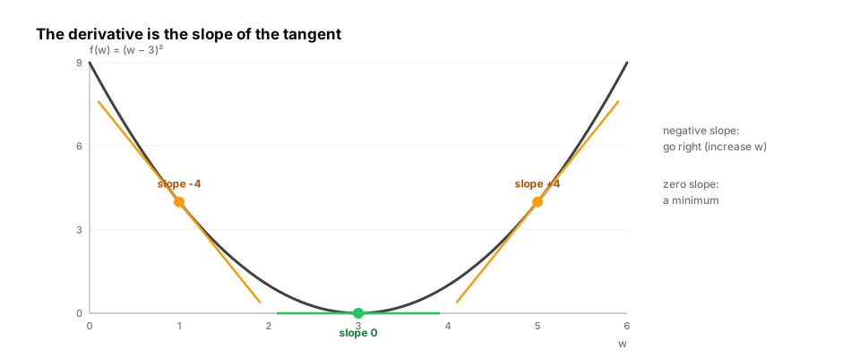
The question. If error = f(w), how do we know which way to move w?
Start from nothing. Nudge the input a tiny amount h and see how much the output changes:
f′(w) ≈ (f(w + h) − f(w)) / h
As h shrinks, this ratio settles on the derivative: the slope of the curve at that point. Positive slope → increasing w increases the error, so move w down. Negative → move w up. Zero → you're at a flat spot (maybe the minimum).
A few rules you'll use constantly:
| Function | Derivative |
|---|---|
c (constant) |
0 |
w² |
2w |
wⁿ |
n·wⁿ⁻¹ |
eʷ |
eʷ |
ln w |
1/w |
a·f(w) + g(w) |
a·f′(w) + g′(w) |
Real-life analogy. A car's speedometer: position is the function, speed is its derivative — how fast position is changing right now.
Worked example.
def f(w):
    return (w - 3) ** 2          # error is smallest at w = 3

def numerical_derivative(fn, w, h=1e-6):
    return (fn(w + h) - fn(w - h)) / (2 * h)   # centred difference: more accurate

for w in [1.0, 3.0, 5.0]:
    print(f"w={w}: slope ≈ {numerical_derivative(f, w):.4f}, exact 2(w-3) = {2 * (w - 3):.1f}")
Common trap. Using a huge h (inaccurate) or a tiny one like 1e-15 (floating-point round-off dominates). Around 1e-5–1e-6 with the centred formula is a good default.
From production
A custom loss layer's analytic gradient disagrees with the numerical estimate (f(w+h) − f(w−h)) / 2h by a factor of exactly 2 at every point.
What's the most likely bug?
Show the answer
C. A missing or extra constant factor in the hand-derived derivative (e.g. forgetting the 2 in d/dw of w²), which a finite-difference gradient check catches immediately — A consistent factor-of-2 mismatch is a derivation slip, not noise. Comparing analytic gradients against central finite differences at a few random points (a gradient check) is the standard test for any custom op.
2. Partial derivatives and the gradient
The question. Real models have millions of weights. What's "the slope" then?
Start from nothing. With several inputs, change one at a time while holding the others fixed: that's a partial derivative, written ∂f/∂w₁. Stack all the partial derivatives into a vector and you get the gradient, ∇f. The gradient points in the direction of steepest increase; its negative points steepest downhill. That single fact is the basis of training: step against the gradient.
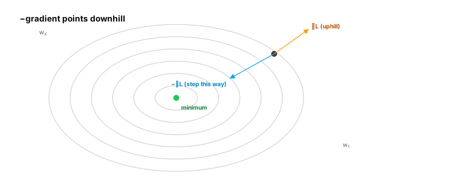
Real-life analogy. Standing on a hillside: the gradient is the compass direction of steepest climb. Walk the opposite way to descend fastest.
Worked example.
import numpy as np

def loss(w):                         # bowl with its minimum at (2, -1)
    return (w[0] - 2) ** 2 + 3 * (w[1] + 1) ** 2

def grad(w):                         # partial derivatives, worked out by hand
    return np.array([2 * (w[0] - 2), 6 * (w[1] + 1)])

def numeric_grad(fn, w, h=1e-6):
    g = np.zeros_like(w)
    for i in range(len(w)):
        e = np.zeros_like(w); e[i] = h
        g[i] = (fn(w + e) - fn(w - e)) / (2 * h)
    return g

w = np.array([0.0, 0.0])
print(grad(w), numeric_grad(loss, w))      # both [-4.  6.]

for step in range(50):                     # gradient descent preview
    w -= 0.1 * grad(w)
print(w.round(4), round(loss(w), 6))       # close to [2, -1], loss ~0
The analytic and numerical gradients agree — that comparison (gradient checking) is how engineers verify a hand-written backward pass.
Quick check
A loss depends on 3 weights: L = (w₁ + 2w₂ − w₃ − 4)². At w = (1, 1, 1), which way should the weights move to reduce L?
Show the answer
D. Opposite to the gradient: the gradient is 2(w₁ + 2w₂ − w₃ − 4)·(1, 2, −1) = (−8, −16, 8), so increase w₁ and w₂ and decrease w₃, with w₂ moving most — Each partial derivative says how sensitive the loss is to that weight. Gradient descent steps against the gradient vector, so weights with larger partials move more.
3. The chain rule: derivatives through a pipeline
The question. A model is many functions stacked: loss(softmax(W x)). How do we get the derivative of the whole chain?
Start from nothing. If y = g(x) and z = f(y), then a small change in x changes y by g′(x) per unit, and each unit of y changes z by f′(y). Multiply:
dz/dx = dz/dy · dy/dx
For a long chain, multiply the local derivatives along the path. When a value feeds into several places, add the contributions from each path.
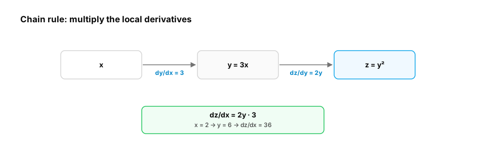
Real-life analogy. Gears: if gear A turns gear B three times per turn, and B turns C twice per turn, then A turns C six times per turn.
Worked example. z = (3x + 1)² at x = 2: y = 3x + 1 = 7, dz/dy = 2y = 14, dy/dx = 3, so dz/dx = 42.
x = 2.0
y = 3 * x + 1
z = y ** 2
dz_dy = 2 * y
dy_dx = 3
print("chain rule:", dz_dy * dy_dx)                                  # 42.0

h = 1e-6
numeric = ((3 * (x + h) + 1) ** 2 - (3 * (x - h) + 1) ** 2) / (2 * h)
print("numerical :", round(numeric, 4))                              # 42.0
From production
A pipeline computes y = log(softmax(z)) and you need dy/dz. A colleague differentiates log and softmax separately and multiplies the results by hand.
What does the chain rule guarantee, and what do frameworks do in practice?
Show the answer
B. The derivative of the composition is the product of the local derivatives, so the colleague's approach is valid; frameworks apply exactly this automatically and often fuse log∘softmax into one numerically stable op — Chain rule: d(f∘g) = f′(g)·g′. Autograd applies it node by node. Fused ops like log_softmax compute the same derivative with better numerical behaviour.
4. Backpropagation: the chain rule, organized
The question. Computing each of a million partial derivatives separately would mean a million forward passes. How do frameworks do it in about the cost of one?
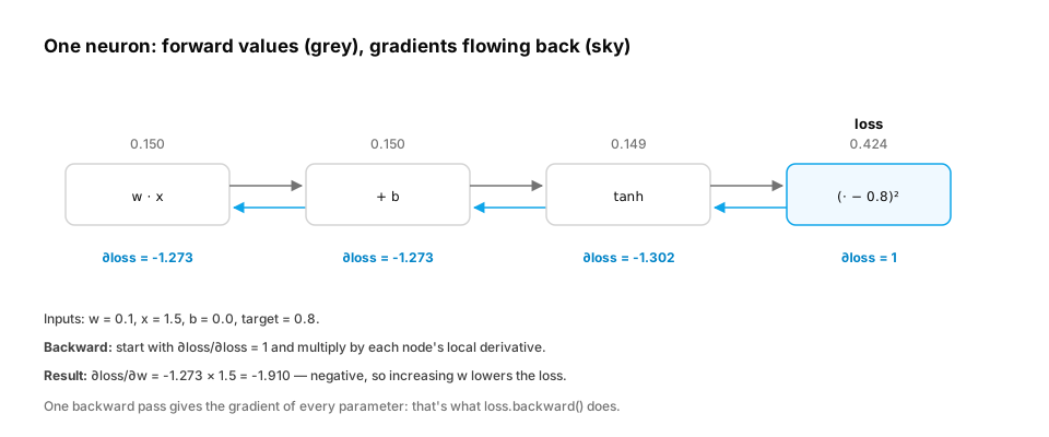
Start from nothing. Record the computation as a graph (a DAG, D1 Data structures §5): each node is a simple operation that knows its own local derivative. Then:
- Forward pass — compute values from inputs to the loss.
- Backward pass — start at the loss with gradient 1, walk the graph in reverse topological order, and at each node multiply the incoming gradient by the local derivative and pass it to the node's inputs (adding where paths merge).
One backward pass gives the gradient for every parameter. That's reverse-mode automatic differentiation, which is what loss.backward() does in PyTorch.
Worked example — a tiny autograd engine (the same idea as PyTorch, in ~40 lines):
import math

class Value:
    def __init__(self, data, parents=(), backward=lambda: None):
        self.data, self.grad = data, 0.0
        self._parents, self._backward = parents, backward

    def __add__(self, other):
        other = other if isinstance(other, Value) else Value(other)
        out = Value(self.data + other.data, (self, other))
        def backward():
            self.grad += out.grad          # d(a+b)/da = 1
            other.grad += out.grad
        out._backward = backward
        return out

    def __mul__(self, other):
        other = other if isinstance(other, Value) else Value(other)
        out = Value(self.data * other.data, (self, other))
        def backward():
            self.grad += other.data * out.grad   # d(ab)/da = b
            other.grad += self.data * out.grad
        out._backward = backward
        return out

    def tanh(self):
        t = math.tanh(self.data)
        out = Value(t, (self,))
        def backward():
            self.grad += (1 - t * t) * out.grad
        out._backward = backward
        return out

    def __sub__(self, other):
        return self + (other * -1 if isinstance(other, Value) else Value(-other))

    def backward(self):
        order, seen = [], set()
        def visit(v):
            if v not in seen:
                seen.add(v)
                for p in v._parents:
                    visit(p)
                order.append(v)
        visit(self)
        self.grad = 1.0
        for v in reversed(order):
            v._backward()

# One neuron learns: predict 0.8 from input 1.5
w, b = Value(0.1), Value(0.0)
x, target = 1.5, 0.8
for step in range(60):
    pred = (w * x + b).tanh()
    err = pred - target
    loss = err * err
    w.grad = b.grad = 0.0
    loss.backward()
    w.data -= 0.5 * w.grad
    b.data -= 0.5 * b.grad
print(f"prediction {(w * x + b).tanh().data:.3f} (target {target}), loss {loss.data:.6f}")
Common traps
- Forgetting to reset gradients each step — they accumulate (
+=). In PyTorch that'soptimizer.zero_grad(). - Thinking backprop is a learning algorithm. It only computes gradients; the optimizer (next lesson) uses them.
In production / interviews. Interview question: "Why is reverse-mode autodiff used for neural networks instead of forward-mode?" (One scalar loss, millions of inputs: reverse mode gets all gradients in one backward pass.)
From production
Training a 10-layer network, you log gradient norms per layer: the last layer's is 1e-1 and the first layer's is 1e-9.
What is this, and what are standard remedies?
Show the answer
C. Vanishing gradients: the backward pass multiplies by each layer's local derivative, which shrinks the signal; use ReLU-family activations, careful initialisation, normalisation layers and residual connections — Backprop multiplies local Jacobians layer by layer. If they're mostly < 1 (saturating sigmoids, poor init), gradients shrink geometrically towards the input. The listed fixes keep the per-layer factors near 1.
5. When gradients vanish or explode
The question. Why did deep networks refuse to train for years?
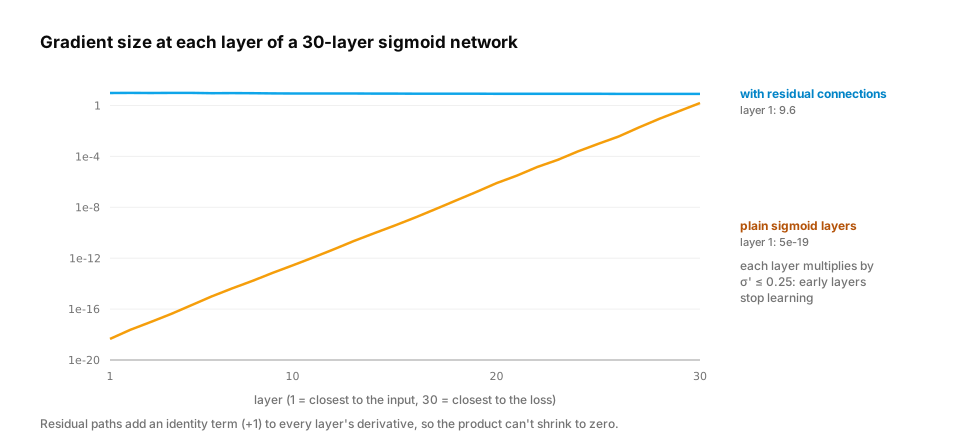
Start from nothing. Backprop multiplies many local derivatives together. If most are below 1 (like the sigmoid's, which never exceeds 0.25), the product shrinks toward zero through many layers — vanishing gradients: early layers stop learning. If most are above 1, it blows up — exploding gradients: training diverges.
Fixes you'll meet in D4: ReLU-family activations (derivative 1 for positive inputs), careful weight initialization, normalization layers, residual (skip) connections that give gradients a short path, and gradient clipping for explosions.
Worked example.
import numpy as np

sigmoid_max_slope = 0.25
for depth in [5, 10, 20, 50]:
    print(f"{depth:>2} sigmoid layers: gradient scaled by at most {sigmoid_max_slope ** depth:.2e}")

# Gradient clipping: rescale if the norm is too big
g = np.array([30.0, 40.0])                    # norm 50
max_norm = 5.0
norm = np.linalg.norm(g)
clipped = g * min(1.0, max_norm / norm)
print(clipped, np.linalg.norm(clipped))      # [3. 4.] 5.0
Quick check
A 40-layer network with sigmoid activations trains its last layers but its first layers barely change. Why?
Show the answer
C. Backprop multiplies many derivatives below 0.25 together, so gradients vanish towards the early layers — The chain rule multiplies per-layer derivatives; sigmoid's maximum derivative is 0.25, so the product shrinks exponentially with depth.
Check yourself
- Recall: In which direction do we update weights relative to the gradient?
- Apply:
z = (2x − 1)³. What isdz/dxatx = 1? - Predict: In the tiny autograd engine, what happens if you remove
w.grad = b.grad = 0.0? - Apply: How would you test a hand-written gradient for a new layer?
- Diagnose: First-layer gradient norms are a million times smaller than last-layer norms. What's happening?
Answers
- Opposite to it (gradient descent):
w ← w − lr · ∇loss. 3(2x − 1)² · 2 = 6(2x − 1)²→ at x = 1,6 · 1 = 6.- Gradients accumulate across steps, so updates grow larger each step and training oscillates or diverges.
- A gradient check: compare it with the central finite difference (f(w+h) − f(w−h)) / 2h at a few random points; they should agree to several digits.
- Vanishing gradients: multiplying many small local derivatives shrinks the signal on its way back. Use non-saturating activations, good initialisation, normalisation and residual connections.
Exercise
Add __pow__ (integer powers) and relu() to the Value class, then train two weights w1, w2 so that relu(w1·x1 + w2·x2) fits three data points ([1,2]→3), ([2,1]→3), ([3,3]→6). Verify your gradients against a numerical gradient check before training.
Solution
class Value:
    def __init__(self, data, parents=()):
        self.data, self.grad, self._parents, self._backward = data, 0.0, parents, lambda: None
    def __add__(self, o):
        o = o if isinstance(o, Value) else Value(o)
        out = Value(self.data + o.data, (self, o))
        def bw(): self.grad += out.grad; o.grad += out.grad
        out._backward = bw; return out
    __radd__ = __add__          # lets sum() start from 0: 0 + Value
    def __mul__(self, o):
        o = o if isinstance(o, Value) else Value(o)
        out = Value(self.data * o.data, (self, o))
        def bw(): self.grad += o.data * out.grad; o.grad += self.data * out.grad
        out._backward = bw; return out
    def __pow__(self, n):
        out = Value(self.data ** n, (self,))
        def bw(): self.grad += n * self.data ** (n - 1) * out.grad
        out._backward = bw; return out
    def relu(self):
        out = Value(max(0.0, self.data), (self,))
        def bw(): self.grad += (self.data > 0) * out.grad
        out._backward = bw; return out
    def backward(self):
        order, seen = [], set()
        def visit(v):
            if v not in seen:
                seen.add(v); [visit(p) for p in v._parents]; order.append(v)
        visit(self); self.grad = 1.0
        for v in reversed(order): v._backward()

data = [((1, 2), 3), ((2, 1), 3), ((3, 3), 6)]
def total_loss(w1, w2):
    return sum(((w1 * x1 + w2 * x2).relu() + (-y)) ** 2 for (x1, x2), y in data)

w1, w2 = Value(0.5), Value(0.5)
L = total_loss(w1, w2); L.backward()
h = 1e-6
num_w1 = (total_loss(Value(0.5 + h), Value(0.5)).data - total_loss(Value(0.5 - h), Value(0.5)).data) / (2 * h)
print(f"grad check w1: autograd {w1.grad:.4f} vs numerical {num_w1:.4f}")

for _ in range(200):
    w1.grad = w2.grad = 0.0
    L = total_loss(w1, w2); L.backward()
    w1.data -= 0.01 * w1.grad; w2.data -= 0.01 * w2.grad
print(f"w1={w1.data:.3f}, w2={w2.data:.3f}, loss={L.data:.5f}")   # ~1, ~1
This unlocks:
- Probability & statistics — what the loss should measure when outputs are uncertain.
- Optimization — smarter ways to use gradients than a fixed step (momentum, Adam).
- D4 Neural network fundamentals — backprop through real layers; why ReLU and residuals help.
Sources: Goodfellow, Bengio & Courville, Deep Learning (ch. 4, 6.5); Karpathy, micrograd; Baydin et al., Automatic Differentiation in Machine Learning: a Survey (2018); PyTorch docs — "Autograd mechanics".