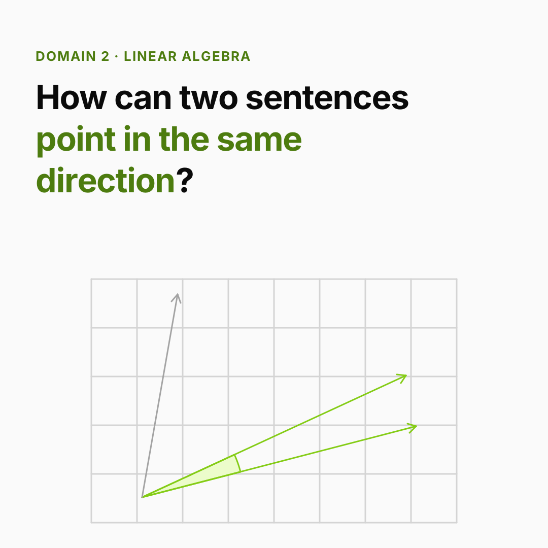
You already know: a vector is a list of scores, and similar meanings point in similar directions (Bridge D1 → D2); NumPy stores numbers packed side by side (Python internals §3).
Why this matters for Atlas. Every modern AI model is, underneath, a long chain of vector and matrix operations. Embeddings are vectors, model layers are matrices, and attention — the heart of every LLM — is three matrix multiplications and a softmax. Learn these few operations and the rest of the course reads like a story.
1. Vectors: a list of numbers, an arrow, a point
The question. What is a vector, and why can it represent a word, an image or a student?
Start from nothing. A vector is an ordered list of numbers: [3, 1]. You can read it three ways, all useful:
- A list of features —
[hours_studied, quizzes_passed]. - A point in space — 3 steps right, 1 up.
- An arrow from the origin to that point, with a length and a direction.
The number of entries is its dimension. Real embeddings have hundreds or thousands of dimensions; we can't draw them, but the same rules apply in 2-D and in 4,096-D.
Two basic operations:
- Add vectors entry by entry:
[3,1] + [1,2] = [4,3](walk one arrow, then the other). - Scale by a number:
2 × [3,1] = [6,2](same direction, twice as long).
Length (norm): ‖v‖ = √(v₁² + v₂² + …) — Pythagoras in any number of dimensions.
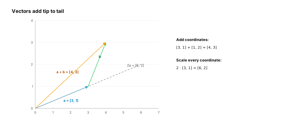
Real-life analogy. A recipe as a vector: [flour, sugar, eggs]. Doubling the recipe scales the vector; combining two recipes adds them.
Worked example.
import numpy as np

a = np.array([3.0, 1.0])
b = np.array([1.0, 2.0])
print(a + b)                       # [4. 3.]
print(2 * a)                       # [6. 2.]
print(np.linalg.norm(a))           # 3.162... = sqrt(3**2 + 1**2)
unit = a / np.linalg.norm(a)       # same direction, length 1 ("normalized")
print(unit, np.linalg.norm(unit))  # [0.949 0.316] 1.0
Common trap. Treating dimensions as interchangeable. Entry 0 must mean the same thing in every vector you compare — that's why all embeddings from one model share one "coordinate system", and embeddings from two different models can't be compared directly.
From production
A recommendation team stores each user as a vector of [age, monthly_spend_in_rupees, sessions_per_week] and finds that 'similar users' are just users with similar spend.
What's the most likely cause?
Show the answer
D. The features are on wildly different scales, so spend (thousands) dominates distances and dot products; standardise each feature (or use learned embeddings) before comparing — Geometry treats every coordinate equally. A feature measured in thousands swamps one measured in units, so 'closeness' means 'similar spend'. Scaling features (z-scores) or learning an embedding puts them on comparable footing.
2. The dot product: how aligned are two vectors?
The question. How do we turn "these two meanings are similar" into one number?
Start from nothing. Multiply matching entries and add them up:
a · b = a₁b₁ + a₂b₂ + … + aₙbₙ
If both vectors have large values in the same places, the sum is large; if one is large where the other is negative, terms cancel. Geometrically:
a · b = ‖a‖ ‖b‖ cos θ
where θ is the angle between them. Dividing out the lengths gives cosine similarity, a pure measure of direction from −1 (opposite) through 0 (unrelated / perpendicular) to 1 (same direction).
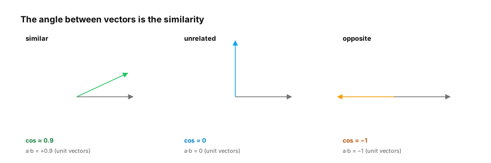
Real-life analogy. Two friends rating the same five films from −2 to +2. Multiply their ratings film by film and add them: big and positive means similar taste; near zero means unrelated taste; negative means opposite taste.
Worked example — finding the most relevant lesson for a question:
import numpy as np

# toy 4-D "embeddings": [memory, networking, maths, hardware]
lessons = {
    "Virtual memory & paging": np.array([0.9, 0.1, 0.1, 0.6]),
    "TCP and TLS":             np.array([0.1, 0.9, 0.0, 0.2]),
    "Dot products":            np.array([0.0, 0.0, 0.9, 0.1]),
    "GPU memory hierarchy":    np.array([0.8, 0.0, 0.1, 0.9]),
}
question = np.array([0.7, 0.0, 0.1, 0.8])   # "why does my GPU run out of memory?"

def cosine(a, b):
    return a @ b / (np.linalg.norm(a) * np.linalg.norm(b))

ranked = sorted(lessons, key=lambda k: cosine(question, lessons[k]), reverse=True)
for name in ranked:
    print(f"{cosine(question, lessons[name]):.3f}  {name}")
Math check. [2,1] · [3,1] = 6 + 1 = 7; [2,1] · [−1,2] = −2 + 2 = 0 → perpendicular.
Common traps
- Comparing raw dot products of vectors with different lengths: long vectors win just for being long. Normalize (cosine) unless the model was trained for raw dot products.
- Thinking cosine 0.8 means "80% similar". It's an angle measure, and typical values depend heavily on the embedding model.
In production / interviews. Vector databases (D8) are, at their core, very fast "find the largest dot products" engines. Interview question: "When would you use dot product vs cosine similarity for retrieval?"
From production
Two embedding models are compared by raw dot product. Model B's top results are dominated by long, generic documents, whatever the query.
What's the likely reason, and the usual fix?
Show the answer
B. Dot product grows with vector length, and B's embeddings for long or generic documents have larger norms; normalise to unit length (cosine similarity), or use the similarity the model was trained with — a·b = |a||b|cos θ. Unless vectors are normalised, larger-norm vectors win regardless of direction. Many embedding models are trained for cosine similarity, so either normalise or follow the model card.
3. Matrices: transformations and stacks of vectors
The question. A model layer takes a 768-number vector and produces another vector. What does it actually do?
Start from nothing. A matrix is a grid of numbers with shape (rows, cols). Two ways to see it:
- A stack of vectors — e.g. 1,000 lesson embeddings as a
(1000, 4)matrix. - A function that transforms vectors — multiplying
W @ xtakes each row ofW, dot-products it withx, and outputs one number per row. A(3, 4)matrix turns 4-D vectors into 3-D vectors: it can rotate, stretch, squash or mix features.
Matrix multiplication A @ B is "every row of A dot every column of B". The shapes must line up: (m, k) @ (k, n) → (m, n). The inner k must match and disappears.
A neural-network layer is exactly this: y = W x + b, followed by a simple nonlinearity (D4).
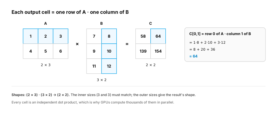
Real-life analogy. A matrix is a recipe-to-nutrition converter: each row says how much protein, fat or sugar each ingredient adds. Multiply it by a recipe vector to get the nutrition vector.
Worked example.
import numpy as np

# Score ALL lessons against ALL questions at once: (questions × dims) @ (dims × lessons)
lessons = np.array([[0.9, 0.1, 0.1, 0.6],
                    [0.1, 0.9, 0.0, 0.2],
                    [0.0, 0.0, 0.9, 0.1]])          # (3 lessons, 4 dims)
questions = np.array([[0.7, 0.0, 0.1, 0.8],
                      [0.0, 0.8, 0.1, 0.1]])        # (2 questions, 4 dims)

scores = questions @ lessons.T                      # (2, 4) @ (4, 3) -> (2, 3)
print(scores.round(2))
print("best lesson per question:", scores.argmax(axis=1))   # [0 1]

# A layer: project 4-D features to 2-D
W = np.array([[1.0, 0.0, 0.0, 1.0],     # "systems-ness"
              [0.0, 1.0, 1.0, 0.0]])    # "theory-ness"
print(W @ questions[0])                  # [1.5 0.1]
Math. Cost of (m, k) @ (k, n): m × n × k multiply-adds. For a 4,096 × 4,096 layer on a batch of 1,000 tokens: 4,096 × 4,096 × 1,000 ≈ 1.7 × 10¹⁰ — which is why GPUs (thousands of parallel multipliers) matter.
Common traps
A @ B ≠ B @ Ain general — order matters.*in NumPy is element-wise,@is matrix multiplication. Mixing them up gives wrong answers with no error if shapes happen to broadcast.
Quick check
A layer computes y = W x with W of shape (3072, 768). What does it do to a 768-dimensional input vector?
Show the answer
C. Maps it to a 3,072-dimensional vector: each output coordinate is a dot product of one row of W with x — Matrix-vector multiplication is a stack of dot products, one per row. A (3072, 768) matrix takes ℝ⁷⁶⁸ to ℝ³⁰⁷², like the expansion in a transformer's MLP block.
4. Tensors, shapes and broadcasting
The question. A batch of 32 sentences, each 128 tokens, each token a 768-D vector. What's that?
Start from nothing. A tensor is just an array with any number of dimensions:
- 0-D scalar
5· 1-D vector(768,)· 2-D matrix(128, 768)· 3-D(32, 128, 768)= (batch, sequence, features).
Most bugs in ML code are shape bugs. Reading shapes is a core skill: for any operation, write the input and output shapes.
Broadcasting lets NumPy/PyTorch combine arrays of different shapes by stretching size-1 dimensions without copying: adding a bias of shape (768,) to activations of shape (32, 128, 768) adds it to every token in every sentence.
Rule: compare shapes from the right; each pair of dimensions must be equal, or one of them must be 1.
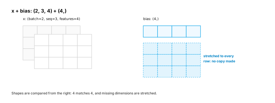
Worked example.
import numpy as np

batch, seq, dim = 2, 3, 4
x = np.arange(batch * seq * dim, dtype=float).reshape(batch, seq, dim)
bias = np.array([100.0, 200.0, 300.0, 400.0])        # (4,)
print((x + bias).shape)                               # (2, 3, 4) — bias added to every token

W = np.ones((dim, 2))                                 # project 4 -> 2 features
y = x @ W                                             # (2, 3, 4) @ (4, 2) -> (2, 3, 2)
print(y.shape)

mean_per_sentence = x.mean(axis=1)                    # average over tokens -> (2, 4)
print(mean_per_sentence.shape)

try:
    x + np.ones(3)                                    # (2,3,4) vs (3,): 4 vs 3 mismatch
except ValueError as e:
    print("broadcast error:", e)
Common trap. Broadcasting that succeeds by accident: adding shape (3, 1) to (3,) yields (3, 3), not an error. Assert shapes in your code.
From production
A per-feature normalisation is written as X - mean where X has shape (32, 128, 768) and mean was computed with X.mean(axis=0), giving shape (128, 768).
What did this compute?
Show the answer
A. It subtracted, for each (token position, feature), the mean across the 32 sequences in the batch; per-token feature normalisation (like LayerNorm) needs the mean over the last axis with keepdims=True, shape (32, 128, 1) — Broadcasting made the shapes compatible, so no error was raised, but the statistic is over the wrong axis. Write down which axis each statistic should reduce over, and keep the reduced dimension (keepdims=True) so the broadcast is explicit.
5. Attention in one formula
The question. How does an LLM decide which earlier words matter for the next word?
Start from nothing. Each token produces three vectors through three learned matrices:
- a query
q— "what am I looking for?", - a key
k— "what do I contain?", - a value
v— "what do I pass on if chosen?".
For one token, dot its query with every token's key (relevance scores), divide by √d to keep scores in a sensible range, turn them into weights that sum to 1 with softmax, and take the weighted average of the values. For all tokens at once:
Attention(Q, K, V) = softmax(Q Kᵀ / √d) V
That's two matrix multiplications and a softmax. Everything in D5 builds on this.
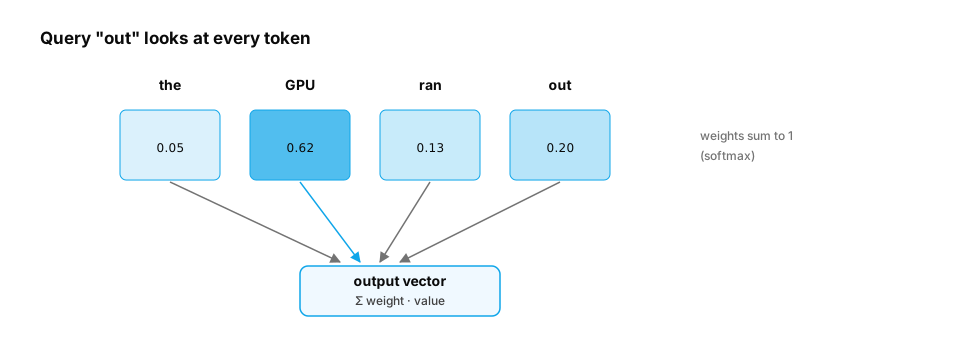
Real-life analogy. Searching a library: your question (query) is compared with each book's catalogue card (key), and you read mostly from the best matches (values), weighted by how well they matched.
Worked example.
import numpy as np

def softmax(z, axis=-1):
    z = z - z.max(axis=axis, keepdims=True)          # stability: avoid huge exponents
    e = np.exp(z)
    return e / e.sum(axis=axis, keepdims=True)

rng = np.random.default_rng(0)
tokens = ["the", "GPU", "ran", "out"]
d = 8
X = rng.normal(size=(len(tokens), d))                # token embeddings (4, 8)
Wq, Wk, Wv = (rng.normal(size=(d, d)) for _ in range(3))

Q, K, V = X @ Wq, X @ Wk, X @ Wv                     # each (4, 8)
weights = softmax(Q @ K.T / np.sqrt(d))              # (4, 4), each row sums to 1
out = weights @ V                                    # (4, 8)

print(np.round(weights[-1], 2), "<- how much 'out' attends to each token")
print(weights.sum(axis=1))                           # [1. 1. 1. 1.]
print(out.shape)
Why divide by √d? If entries of q and k are roughly unit-variance, their dot product has variance about d. Large scores push softmax into near one-hot outputs with tiny gradients; dividing by √d brings the variance back to about 1.
Quick check
Why is attention scaled by 1/√d before the softmax?
Show the answer
D. Dot products of d-dimensional vectors with roughly unit-variance entries have variance about d, so without scaling the softmax saturates at large d (near one-hot), and gradients through it vanish — Each score is a sum of d products. Dividing by √d keeps the scores' variance about 1 regardless of width, so the softmax stays in a range where it still has useful gradients.
6. Low rank: why big matrices can be cheap to adapt
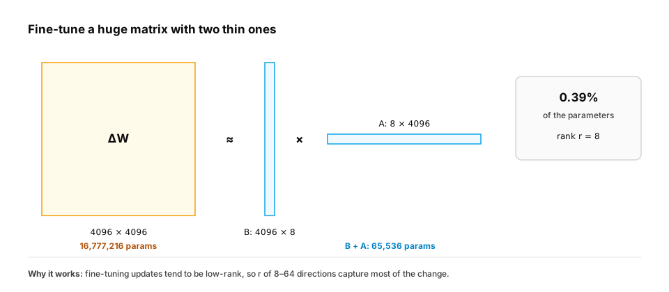
The question. Fine-tuning a 4,096 × 4,096 weight matrix means 16.8 million numbers. Is there a shortcut?
Start from nothing. The rank of a matrix is how many independent directions it really uses. Many useful changes to a model's weights are approximately low rank: they can be written as the product of a tall thin matrix and a short wide one:
ΔW (4096×4096) ≈ B (4096×r) @ A (r×4096), with r = 8 → 2 × 4,096 × 8 = 65,536 numbers instead of 16.8 million (256× fewer).
That's exactly LoRA (D6). The tool that finds the best low-rank approximation is the singular value decomposition (SVD), which also powers PCA (D3).
Worked example.
import numpy as np

rng = np.random.default_rng(1)
n, true_rank = 200, 4
delta = rng.normal(size=(n, true_rank)) @ rng.normal(size=(true_rank, n))  # secretly rank 4
delta += 0.01 * rng.normal(size=(n, n))                                     # plus a little noise

U, S, Vt = np.linalg.svd(delta)
print("top singular values:", S[:6].round(1))        # 4 big ones, then tiny

r = 4
approx = (U[:, :r] * S[:r]) @ Vt[:r]                  # best rank-4 approximation
error = np.linalg.norm(delta - approx) / np.linalg.norm(delta)
print(f"relative error with rank {r}: {error:.4f}")
print(f"params: full {n*n:,} vs low-rank {2*n*r:,}")
Common trap. "Low rank = low quality." It means "few independent directions". When the true change is low rank, the approximation is nearly exact, as the example shows.
Quick check
Two embedding vectors have cosine similarity 0.95 but very different lengths. What does that tell you?
Show the answer
A. They point in almost the same direction (similar meaning) even though their magnitudes differ; cosine ignores length — Cosine similarity is the dot product of the normalized vectors, measuring direction only.
Check yourself
- Recall: What shape does
(32, 128, 768) @ (768, 64)produce? - Apply: Two embeddings have cosine similarity −0.9. What does that suggest?
- Predict: In the attention example, what does each row of
weightssum to, and why? - Diagnose: Why can raw dot-product retrieval favour long or generic documents, and what fixes it?
- Apply: Why does a reduction over the wrong axis often run without an error?
Answers
(32, 128, 64)— the shared 768 disappears.- They point in nearly opposite directions: strongly dissimilar along the features the model uses.
- 1 — softmax turns each row of scores into weights that sum to 1 (a weighted average of the values).
- Dot product grows with vector norm, so large-norm vectors score high in any direction. Normalise to unit length (cosine) or use the similarity the embedding model was trained for.
- Broadcasting stretches size-1 or missing dimensions to fit, so a wrongly shaped statistic can still combine with the tensor. Track shapes and use keepdims=True so the intended axis is explicit.
Exercise
Implement top_k_lessons(question_vec, lesson_matrix, k) using one matrix operation (no Python loop over lessons) that returns the indices of the k most similar lessons by cosine similarity. Then implement single-head attention with a causal mask (each token may only attend to itself and earlier tokens) and check that the first token's weights are [1, 0, 0, 0].
Solution
import numpy as np

def top_k_lessons(q, L, k):
    sims = (L @ q) / (np.linalg.norm(L, axis=1) * np.linalg.norm(q))
    return np.argsort(-sims)[:k]

def causal_attention(X, Wq, Wk, Wv):
    Q, K, V = X @ Wq, X @ Wk, X @ Wv
    scores = Q @ K.T / np.sqrt(Q.shape[-1])
    mask = np.triu(np.ones_like(scores, dtype=bool), k=1)      # True above the diagonal
    scores = np.where(mask, -np.inf, scores)
    scores -= scores.max(axis=-1, keepdims=True)
    w = np.exp(scores); w /= w.sum(axis=-1, keepdims=True)
    return w @ V, w

rng = np.random.default_rng(0)
L = rng.normal(size=(1000, 16)); q = L[42] + 0.05 * rng.normal(size=16)
print(top_k_lessons(q, L, 3))          # lesson 42 first

X = rng.normal(size=(4, 8)); Ws = [rng.normal(size=(8, 8)) for _ in range(3)]
_, w = causal_attention(X, *Ws)
print(np.round(w, 2))                  # first row [1, 0, 0, 0]; upper triangle all 0
This unlocks:
- Calculus — how the numbers inside
Wget learned. - D5 Transformer architecture — multi-head attention built from section 5.
- D6 Parameter-efficient fine-tuning — LoRA from section 6.
- D8 Embeddings — real embedding models and similarity search.
Sources: Strang, Introduction to Linear Algebra; 3Blue1Brown, Essence of Linear Algebra; Vaswani et al., Attention Is All You Need (2017); Hu et al., LoRA (2021); NumPy docs — broadcasting.