VFlash: Fast, Accurate Visual Planning via Flash Primitive Decoding
u_Unrolled
D2: Math, Stats & Optimization · Joint Distributions, the Gaussian, Sampling and the Central Limit Theorem
Phase 1/Domain 2/Lesson 8

Joint Distributions, the Gaussian, Sampling and the Central Limit Theorem

15 min read·Foundational· Unrolled Pro
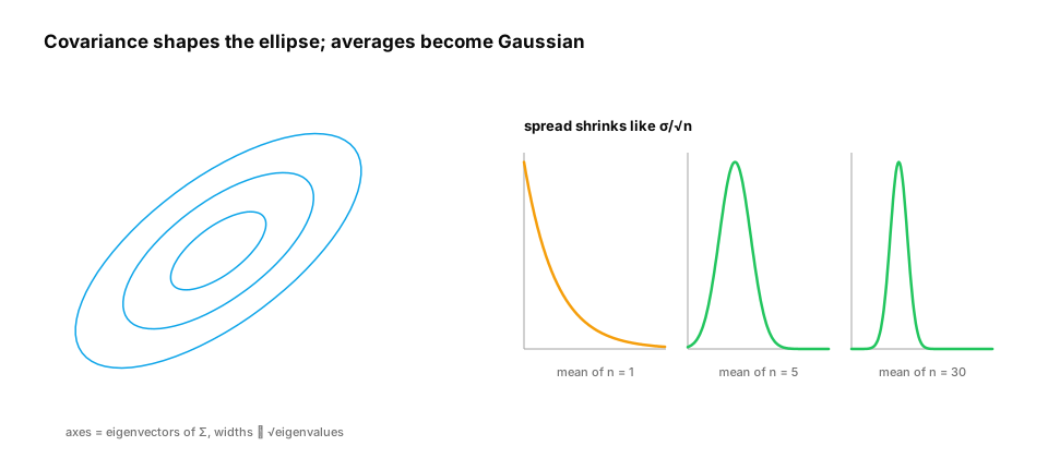
a 2-D Gaussian as an ellipse of contours whose axes are the covariance eigenvectors, with marginal histograms on the sides and a conditional slice; beside it, histograms of the mean of n samples from a skewed distribution becoming bell-shaped as n grows from 1 to 30.
Diagram— a 2-D Gaussian as an ellipse of contours whose axes are the covariance eigenvectors, with marginal histograms on the sides and a conditional slice; beside it, histograms of the mean of n samples from a skewed distribution becoming bell-shaped as n grows from 1 to 30.

You already know: distributions, expectation, variance, Bayes' rule and confidence intervals (Probability); eigenvectors and covariance (Linear systems, SVD and PCA).

Why this matters for Atlas. Real data has many variables at once, so we need joint distributions: how variables vary together (covariance, correlation), what one tells us about another (conditionals), and when they're unrelated (independence). The multivariate Gaussian is the workhorse model for all of it. And the central limit theorem explains why averages (eval accuracy, A/B lifts, mini-batch gradients) are approximately Gaussian with error shrinking like 1/√n, which is the justification behind nearly every error bar in this course.


1. Joint, marginal and conditional distributions

The question. How do you describe two variables together?

Start from nothing. A joint distribution p(x, y) gives probabilities for pairs. Summing (or integrating) out one variable gives a marginal: p(x) = Σ_y p(x, y). Dividing by a marginal gives a conditional: p(y | x) = p(x, y) / p(x). Variables are independent if p(x, y) = p(x)p(y), i.e., knowing x tells you nothing about y. Covariance Cov(X, Y) = E[(X − μx)(Y − μy)] measures linear co-movement; correlation rescales it to [−1, 1]. Zero correlation doesn't imply independence (a relationship can be nonlinear).

That's the preview. The full lesson, with its code and exercises, is part of Unrolled Pro.
Staff AI & Pro Tier Lesson

Unlock "Joint Distributions, the Gaussian, Sampling and the Central Limit Theorem"

The foundations are free forever. Unrolled Pro unlocks the complete lesson, production architectures, and 55 battle-tested ML system design case studies.

Everything included with Pro:
All 234+ Deep-Dive Lessons across transformer internals, inference, RAG & agents
55 Staff-Level ML & System Design Case Studies with mathematical capacity estimates
AI Engineer Sheet & Exercises with worked solutions, self-checks, and code
100 Landmark Research Papers guided walkthroughs & progress tracking
14-Day Money-Back Guarantee — 100% full refund if you aren't satisfied
View Plans & Unlock All Lessons

From ₹167/mo (~$2/mo) · Cancel anytime · Instant activation

100% Risk-Free: 14-day no-questions-asked money-back guarantee