You already know: Python loops, lists, dicts and functions (Python track); NumPy arrays (Python internals).
Why this matters for Atlas. ML maths is mostly a handful of symbols used over and over: functions mapping one space to another, sets and membership, sums and products over indices, and argmax/argmin to pick the best option. The loss of a language model, the definition of attention and the training objective of every model in this course are written this way. This lesson translates each symbol into code, so formulas become something you can run and check.
1. Functions and sets
The question. What does f: ℝⁿ → ℝ mean, and why do papers bother writing it?
Start from nothing. A function f: X → Y maps every element of a domain X to one element of a codomain Y. The signature is a type annotation: f: ℝⁿ → ℝ takes a vector of n real numbers and returns one real number (a loss is such a function); softmax: ℝᵏ → Δᵏ maps k scores to a probability vector. Sets are collections without order or duplicates: x ∈ S means x is in S, A ⊆ B means every element of A is in B, A ∪ B and A ∩ B are union and intersection, {x ∈ S : condition} is a filtered set (a set comprehension), and |S| is the number of elements. Common sets: ℕ (naturals), ℤ (integers), ℝ (reals), ℝⁿ (vectors of n reals), [a, b] (the interval).
import numpy as np

def softmax(z):                                  # softmax: R^k -> simplex (non-negative, sums to 1)
    e = np.exp(z - z.max())
    return e / e.sum()

vocab = {"the", "cat", "sat", "mat"}
sentence = ["the", "cat", "sat", "on", "the", "mat"]
oov = {w for w in sentence if w not in vocab}    # {w in sentence : w not in V}
p = softmax(np.array([2.0, 1.0, 0.1]))
print("out-of-vocabulary set:", oov, "| size |S| =", len(set(sentence)))
print("softmax output:", np.round(p, 3), "sum =", p.sum().round(6), "all >= 0:", bool((p >= 0).all()))
The set comprehension finds {'on'} as the only word outside the vocabulary, and the sentence has 5 distinct words (|S| counts "the" once). The softmax output [0.659 0.242 0.099] sums to 1 with every entry non-negative: it really does land in the probability simplex Δ³, as its signature promised.
The signature you'll read most often: tensor shapes. In ML papers and code, the most common "function signature" is a shape. X ∈ ℝ^{B×T×d} says X is a batch of B sequences, each T tokens long, each token a d-dimensional vector. Matrix products only make sense when inner dimensions agree, so shapes act like types: a mismatch is caught before any maths happens.
import numpy as np

B, T, d = 2, 5, 8                                    # batch, sequence length, model width
rng = np.random.default_rng(0)
X = rng.standard_normal((B, T, d))                   # X ∈ R^{B×T×d}
W_q = rng.standard_normal((d, d))                    # W_Q ∈ R^{d×d}
Q = X @ W_q                                          # (B,T,d)·(d,d) -> (B,T,d)
scores = Q @ Q.transpose(0, 2, 1)                    # (B,T,d)·(B,d,T) -> (B,T,T)
print("X", X.shape, "-> Q", Q.shape, "-> scores", scores.shape)

W_bad = rng.standard_normal((d + 1, d))              # a weight declared as R^{9×8} by mistake
try:
    X @ W_bad
except ValueError:
    print(f"shape error: inner dimensions {X.shape[-1]} and {W_bad.shape[0]} must match")
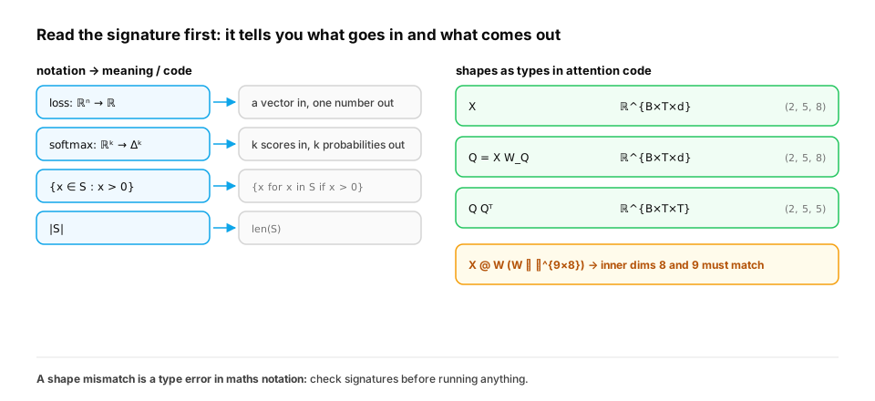
The shapes flow as the notation says: (2, 5, 8) → (2, 5, 8) → (2, 5, 5), one T×T score matrix per sequence. The mis-declared weight fails immediately: inner dimensions 8 and 9 must match.
In production. Writing shapes next to every tensor, in comments, docstrings or type annotations (libraries such as
jaxtypinglet you annotateFloat[Tensor, "batch seq dim"]), is one of the most effective habits in ML engineering. Most model bugs are shape bugs that happen to run: a sum over the wrong axis or a silent broadcast. A signature on paper catches them before they become a wrong number in a training curve.
From production
A paper defines the attention scores S = QKᵀ / √d with Q, K ∈ ℝ^{T×d}. Your implementation produces S with shape (d, d).
What did you most likely do?
Show the answer
A. Computed QᵀK instead of QKᵀ: (d×T)(T×d) gives d×d, while the paper's QKᵀ is (T×d)(d×T) = T×T, one score per pair of tokens — Reading the signature tells you S must be T×T (token-to-token). A d×d result means the transpose is on the wrong factor. Checking shapes against the notation catches this before any training run.
2. Σ and ∏: sums and products over indices
The question. How do you read Σᵢ₌₁ⁿ and ∏ᵢ?
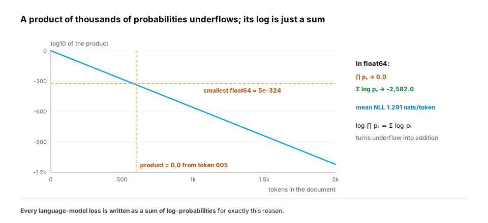
Start from nothing. Σᵢ₌₁ⁿ xᵢ means "for i from 1 to n, add up xᵢ": a loop with an accumulator, or x.sum(). ∏ᵢ means the same with multiplication. Indices can range over sets (Σ_{x∈S}) or conditions (Σ_{i: yᵢ=1}). Two rules make most derivations easy: constants factor out (Σ c·xᵢ = c·Σ xᵢ), and the log of a product is a sum of logs: log ∏ pᵢ = Σ log pᵢ. That last identity is why language models minimize a sum of negative log-probabilities: the probability of a sentence is a product of per-token probabilities, which underflows to zero in floating point for long texts, while its log is a well-behaved sum.
import numpy as np

rng = np.random.default_rng(0)
token_probs = rng.uniform(0.05, 0.6, 2000)            # p(token_t | previous tokens) for a 2,000-token document
product = np.prod(token_probs)
log_sum = np.sum(np.log(token_probs))
print(f"product of probabilities: {product}  (underflowed to zero)")
print(f"sum of log-probabilities: {log_sum:.1f}  -> mean negative log-likelihood {-log_sum / len(token_probs):.3f} nats/token")

# the same sum written three ways
x = rng.standard_normal(5)
loop = 0.0
for i in range(len(x)):
    loop += 3 * x[i]
print(np.isclose(loop, 3 * x.sum()), np.isclose(loop, np.sum(3 * x)))
The product of 2,000 probabilities prints 0.0: it fell below the smallest positive float64 (about 5 × 10⁻³²⁴) partway through the document. The sum of their logs is an ordinary number, -2582.0, which gives a mean negative log-likelihood of 1.291 nats per token. The last line prints True True: the loop, the factored form and the vectorised form agree, which is "constants factor out" checked numerically.
The companion trick: log-sum-exp. Logs fix products, but softmax and its log need a sum of exponentials, and exponentials overflow. Large models routinely produce logits in the hundreds. The identity log Σ exp(zᵢ) = m + log Σ exp(zᵢ − m), with m = max zᵢ, is exact and never overflows:
import numpy as np

z = np.array([1000.0, 999.0, 998.0])                 # large logits are normal for big models
with np.errstate(over="ignore", invalid="ignore"):
    naive = np.log(np.sum(np.exp(z)))                # exp(1000) overflows to inf
m = z.max()
stable = m + np.log(np.sum(np.exp(z - m)))           # log Σ exp(z) = m + log Σ exp(z − m)
print("naive log-sum-exp:", naive)
print("stable log-sum-exp:", round(stable, 4))
print("log-softmax:", np.round(z - stable, 4))
The naive version returns inf. The shifted version returns 1000.4076, and log-softmax [-0.4076 -1.4076 -2.4076] follows by subtraction. Subtracting the maximum changes nothing mathematically, since it cancels between numerator and denominator, but it keeps every exponent at or below 0.
In production. Every deep learning framework implements softmax, log-softmax and cross-entropy with this shift internally (
torch.logsumexp,torch.nn.functional.cross_entropyworking directly on logits). That's why you pass logits to the loss rather than probabilities you computed yourself: computinglog(softmax(z))in two separate steps can producelog(0) = -infand NaN gradients that a fused, stable implementation avoids.
From production
A training run's loss becomes NaN after a few thousand steps. The code computes probs = torch.softmax(logits, -1) and then loss = -torch.log(probs[range(n), y]).mean().
What's the most likely cause and fix?
Show the answer
C. Some probabilities underflow to exactly 0, so log gives -inf and the gradients become NaN; pass the logits to F.cross_entropy (or use log_softmax), which applies the log-sum-exp trick internally — Separate softmax-then-log loses the stability of the fused computation. log_softmax and cross_entropy work in log space, using the max-shift identity, so tiny probabilities never become log(0).
3. argmax, argmin, max and min
The question. What's the difference between max and argmax?
Start from nothing. max_x f(x) is the best value; argmax_x f(x) is where it's achieved (the input). Training is written as θ* = argmin_θ L(θ): we want the parameters, not the loss value. Greedy decoding is argmax_t p(t | context): we want the token, not its probability. In code: np.argmax returns an index; ties are broken by the first occurrence, which is a convention you should know when results look arbitrary.
import numpy as np

vocab = ["Paris", "London", "Rome", "Berlin"]
logits = np.array([3.1, 1.2, 0.4, 3.1])
probs = np.exp(logits) / np.exp(logits).sum()
print(f"max probability {probs.max():.3f}; argmax index {np.argmax(probs)} -> '{vocab[np.argmax(probs)]}' (tie: first wins)")

thetas = np.linspace(-3, 3, 601)
loss = (thetas - 1.25) ** 2 + 0.5
print(f"min loss {loss.min():.3f} at theta* = argmin = {thetas[np.argmin(loss)]:.2f}")
The best probability is 0.451, but argmax returns index 0 ("Paris"): the tie with "Berlin", which has the same logit, goes to the first occurrence. The loss curve's minimum value is 0.500, reached at θ* = 1.25. max and argmax answer different questions about the same curve.
Softmax is a "soft" argmax. argmax is a hard choice with no useful gradient. Nudge the inputs slightly and the output either doesn't change or jumps. Softmax with a temperature T interpolates: high T spreads probability out, and T → 0 approaches the one-hot argmax.
import numpy as np

logits = np.array([2.0, 1.5, 0.3])
for T in (1.0, 0.5, 0.1, 0.01):
    p = np.exp(logits / T - (logits / T).max())
    p /= p.sum()
    print(f"temperature {T:<5} softmax {np.round(p, 3)}")
print("argmax:", np.eye(3)[np.argmax(logits)])
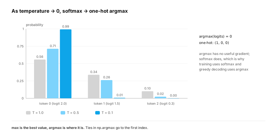
At T = 1 the distribution is [0.559 0.339 0.102]. At 0.5 it sharpens to [0.714 0.263 0.024], at 0.1 it's [0.993 0.007 0.], and at 0.01 it's indistinguishable from argmax's one-hot [1. 0. 0.].
In production. This is exactly the
temperatureparameter in LLM APIs. Decoding divides the model's logits by T before sampling, so T = 0 (or "greedy") means argmax, and higher values sample more diverse tokens. Training always uses the smooth softmax, because gradients must flow. Inference chooses between argmax-like and sampling behaviour per use case: low temperature for extraction and code, higher for brainstorming.
Quick check
A paper writes θ* = argmin_θ Σᵢ ℓ(f_θ(xᵢ), yᵢ). What is θ*?
Show the answer
D. The parameter values that make the total loss over the training examples as small as possible — argmin returns the argument (the parameters) at which the sum of per-example losses is minimized, not the minimum value itself.
4. Reading a real formula
The question. Can you read the cross-entropy loss of a classifier and implement it?
Start from nothing. L(θ) = −(1/N) Σᵢ₌₁ᴺ Σₖ₌₁ᴷ yᵢₖ log p_θ(k | xᵢ). Read it outside in: average over N examples (1/N Σᵢ); inside, sum over K classes (Σₖ); yᵢₖ is 1 for the true class and 0 otherwise (one-hot), so the inner sum picks out the log-probability of the true class; the minus sign turns "maximize log-probability" into "minimize loss". With that reading, the code is two lines.
import numpy as np

rng = np.random.default_rng(1)
N, K = 4, 3
logits = rng.standard_normal((N, K))
y = np.array([0, 2, 1, 2])
p = np.exp(logits) / np.exp(logits).sum(axis=1, keepdims=True)
Y = np.eye(K)[y]                                                  # one-hot y_ik
loss_formula = -(1 / N) * np.sum(Y * np.log(p))                   # literal translation of the double sum
loss_indexed = -np.mean(np.log(p[np.arange(N), y]))               # what the one-hot sum simplifies to
print(f"{loss_formula:.6f} {loss_indexed:.6f}")
Both versions print 0.978593: the literal double sum and the simplified "pick the true class's log-probability" agree, which confirms the reading.
Now the formula at the centre of every LLM. The attention operation from "Attention Is All You Need" (Vaswani et al., 2017) is written Attention(Q, K, V) = softmax(QKᵀ / √d) V. Read it the same way, outside in: a softmax of something, times V. The something is QKᵀ (all query–key dot products), scaled by 1/√d.
import numpy as np

rng = np.random.default_rng(3)
T, d = 4, 8
Q, K, V = (rng.standard_normal((T, d)) for _ in range(3))

def softmax(S):
    E = np.exp(S - S.max(axis=-1, keepdims=True))
    return E / E.sum(axis=-1, keepdims=True)

A = softmax(Q @ K.T / np.sqrt(d))                    # Attention(Q,K,V) = softmax(QKᵀ / √d) V
out = A @ V
print("weights shape", A.shape, "| each row sums to 1:", np.allclose(A.sum(axis=1), 1))
print("output shape", out.shape)
print("row 0 weights:", np.round(A[0], 3))
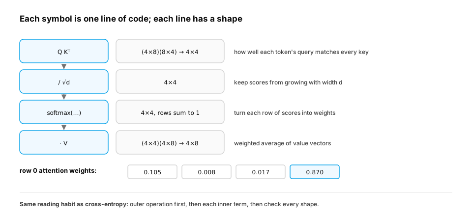
The weights matrix is (4, 4) with every row summing to 1 (True), and the output is (4, 8), one new vector per token. Token 0 puts 0.87 of its attention on token 3 and very little elsewhere: each output row is a weighted average of the value vectors.
In production. Reading papers this way, by writing the shapes and a few lines of NumPy, is how engineers check that an implementation matches its paper before trusting it. Library code adds masking (causal attention sets future positions to −∞ before the softmax), multiple heads and fused kernels. The skeleton is still these three lines (Transformer architecture, in the LLM path).
Quick check
In softmax(QKᵀ / √d) V, along which axis is the softmax taken, and why?
Show the answer
C. Over the last axis (the keys) of the T×T score matrix, so each query's weights over all tokens sum to 1 — Each row is one query's scores against every key. Normalising across that row turns the scores into weights for a weighted average of the value vectors. The wrong axis would mix queries, and the attention would be meaningless.
Check yourself
- What does
f: ℝⁿ → ℝtell you about f? - Translate
{x ∈ S : x > 0}and|S|into Python. - Why do models minimize a sum of log-probabilities instead of a product of probabilities?
- What's the difference between
max_x f(x)andargmax_x f(x)? - In the cross-entropy formula, what does the one-hot yᵢₖ do?
- Why do frameworks compute log-softmax as z − (m + log Σ exp(z − m)) rather than log(softmax(z))?
Answers
- It takes a vector of n real numbers and returns one real number.
{x for x in S if x > 0}andlen(S).- Products of many probabilities underflow to zero; logs turn them into sums that stay well-scaled (and are easier to differentiate).
- The first is the best value; the second is the input that achieves it.
- It selects the log-probability of the true class, so the inner sum has a single non-zero term.
- exp of large logits overflows and tiny probabilities underflow to 0 (giving log 0 = −∞). Subtracting the max keeps every exponent ≤ 0 and keeps the computation in log space.
Exercise
Implement, from their formulas, (a) the mean squared error (1/N) Σᵢ (ŷᵢ − yᵢ)², (b) the log-likelihood of a dataset under a Bernoulli model with parameter q, Σᵢ [yᵢ log q + (1 − yᵢ) log(1 − q)], and (c) q* = argmax_q of that log-likelihood over a grid. Check that q* equals the fraction of ones in the data.
Solution
import numpy as np

rng = np.random.default_rng(2)
y_hat, y_true = rng.standard_normal(10), rng.standard_normal(10)
mse = (1 / len(y_true)) * np.sum((y_hat - y_true) ** 2)
print(f"MSE {mse:.4f}")

y = (rng.random(200) < 0.3).astype(float)
def log_likelihood(q):
    return np.sum(y * np.log(q) + (1 - y) * np.log(1 - q))
grid = np.linspace(0.01, 0.99, 981)
q_star = grid[np.argmax([log_likelihood(q) for q in grid])]
print(f"argmax q = {q_star:.3f}, fraction of ones = {y.mean():.3f}")
The grid search lands on the fraction of ones in the data, which is the maximum-likelihood estimate you'd get by setting the derivative to zero (the Probability lesson derives it). Translating notation directly into code like this is the fastest way to check you've read a formula correctly.
This unlocks:
- Linear algebra — vectors and matrices, written in this notation.
- Probability and statistics — distributions, likelihoods and expectations as sums.
Sources: Goodfellow, Bengio & Courville, Deep Learning, Notation section (2016); Deisenroth, Faisal & Ong, Mathematics for Machine Learning (2020), ch. 1–2; Strang, Introduction to Linear Algebra.