You already know: vectors, dot products and matrix multiplication as a transformation (Linear algebra); reading Σ and argmin notation (Maths notation).
Why this matters for Atlas. Three questions recur across ML: can this system be solved, and is the answer unique? (rank and inverses: least squares, redundant features), what does this matrix do when applied again and again? (eigenvalues: exploding and vanishing gradients, RNN stability, power iteration, Markov chains), and which directions matter? (eigenvectors of covariance matrices, leading to PCA in the next lesson). This lesson builds each from first principles with NumPy checks.
1. Systems of equations and least squares
The question. Given features X and targets y, can we find weights w with Xw = y?
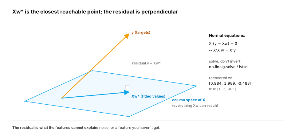
Start from nothing. Xw = y is a system of linear equations: one equation per row (example), one unknown per column (weight). If X is square and invertible, w = X⁻¹y exactly. In ML, X is usually tall (more examples than features) and there's no exact solution, so we solve least squares: w* = argmin_w ‖Xw − y‖², whose solution satisfies the normal equations XᵀX w = Xᵀy. In practice, never form the inverse explicitly: use a solver (np.linalg.solve, lstsq) which is faster and numerically safer.
import numpy as np

rng = np.random.default_rng(0)
X = np.c_[np.ones(100), rng.standard_normal((100, 2))]          # bias + 2 features
w_true = np.array([1.0, 2.0, -0.5])
y = X @ w_true + 0.1 * rng.standard_normal(100)

w_normal = np.linalg.solve(X.T @ X, X.T @ y)                    # normal equations
w_lstsq, *_ = np.linalg.lstsq(X, y, rcond=None)                 # QR/SVD-based solver
print("normal equations:", np.round(w_normal, 3), "| lstsq:", np.round(w_lstsq, 3), "| true:", w_true)
Both solvers recover [0.984 1.989 -0.483] against true weights [1, 2, -0.5]. The small gaps are the 0.1 noise in y: with 100 examples, least squares can't tell noise apart from signal.
In production. Linear least squares is still everywhere in ML systems: calibration layers, linear probes on frozen embeddings, baselines that every fancier model must beat, and fast refits inside feature pipelines. Libraries solve it with QR or SVD factorisations, never an explicit inverse. When you see
inv(X.T @ X) @ X.T @ yin code review, the safe replacement isnp.linalg.lstsq(X, y)orscipy.linalg.lstsq.
From production
A pricing model is refit nightly with w = np.linalg.inv(X.T @ X) @ X.T @ y. One night the weights come out as huge numbers and NaNs, after a new feature was added.
What's the most robust change?
Show the answer
C. Use a least-squares solver (np.linalg.lstsq or a QR/SVD-based routine), check the rank and condition number of X, and add ridge regularisation if features are nearly dependent — Explicit inversion amplifies rounding errors and fails outright when the new feature makes XᵀX (nearly) singular. Solvers based on QR/SVD are stable, and conditioning checks tell you when the data itself is the problem.
2. Rank: redundant information
The question. What happens if one feature is a combination of others?
Start from nothing. The rank of a matrix is the number of linearly independent columns (equivalently rows): the dimension of the space its outputs can reach. If a feature is a linear combination of others (price in dollars and price in cents), X loses rank, XᵀX becomes singular (not invertible), and infinitely many weight vectors fit equally well. Nearly dependent features (multicollinearity) make XᵀX ill-conditioned: tiny changes in data swing the weights wildly. The condition number (ratio of largest to smallest singular value) measures this; regularization (ridge) fixes it by adding λI, making the matrix well conditioned.
import numpy as np

rng = np.random.default_rng(1)
a = rng.standard_normal(200)
X_dup = np.c_[np.ones(200), a, 100 * a]                          # same feature in two units
X_near = np.c_[np.ones(200), a, a + 1e-4 * rng.standard_normal(200)]
for name, X in [("exact duplicate", X_dup), ("near duplicate", X_near)]:
    print(f"{name:<16} rank {np.linalg.matrix_rank(X)} of {X.shape[1]}, condition number of X^T X {np.linalg.cond(X.T @ X):.1e}")
y = 3 * a + 0.1 * rng.standard_normal(200)
for trial in range(2):
    noise = 0.01 * rng.standard_normal(200)
    w = np.linalg.lstsq(X_near, y + noise, rcond=None)[0]
    w_ridge = np.linalg.solve(X_near.T @ X_near + 1.0 * np.eye(3), X_near.T @ (y + noise))
    print(f"tiny data change {trial}: least squares w = {np.round(w, 1)}, ridge w = {np.round(w_ridge, 2)}")
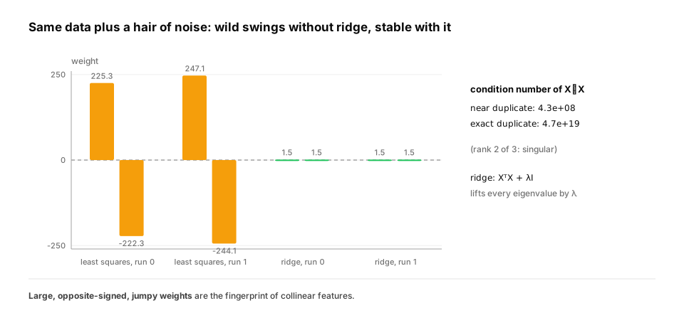
With nearly duplicate features, least squares produces huge opposite weights (around +230 and −230 for a true effect of 3) that shift by twenty units when the data changes by a hair; ridge splits the effect stably, 1.5 on each copy. Rank and conditioning explain why regularization (D3) and feature deduplication matter.
The exact duplicate (the same feature in two units) has rank 2 of 3 and a condition number around 4.7e+19, effectively singular. The near duplicate is technically full rank, but its condition number of 4.3e+08 is what makes the weights swing from 225.3 / -222.3 to 247.1 / -244.1.
In production. Collinearity is common in real feature sets: the same metric logged by two systems, a total next to its components, one-hot encodings that include every category plus a bias. Its symptom is a model that predicts fine but whose coefficients are huge, flip sign between retrains, and mean nothing. That matters as soon as anyone reads the weights for explanations or uses them for decisions. Check the condition number, drop or combine duplicates, or regularise.
From production
A churn model's coefficient on monthly_spend is +4,200 this week and −3,900 last week, while accuracy is identical. The feature set also includes annual_spend.
What's going on?
Show the answer
D. monthly_spend and annual_spend are nearly collinear, so XᵀX is ill-conditioned: many weight combinations fit equally well, and small data changes swing them; drop one, combine them, or use ridge — With near-duplicate features, the data only pins down their combined effect. Individual weights become unstable even though predictions don't change, which is exactly the instability the lesson's experiment shows.
3. Eigenvectors and eigenvalues
The question. Are there directions a matrix only stretches?
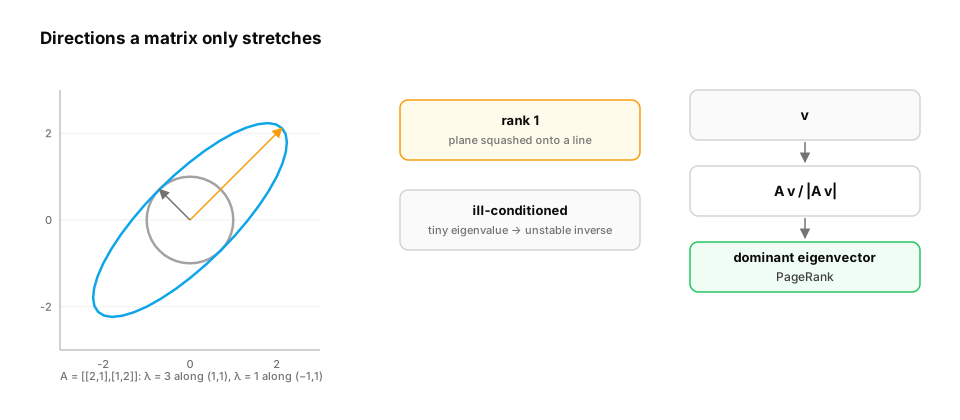
Start from nothing. An eigenvector v of a square matrix A satisfies Av = λv: applying A only scales v, by the eigenvalue λ. Symmetric matrices (like covariance matrices) have real eigenvalues and orthogonal eigenvectors, so A = QΛQᵀ: rotate into the eigenbasis, scale each axis, rotate back. Applying A k times scales each eigen-direction by λᵏ, which is the whole story of exploding (|λ| > 1) and vanishing (|λ| < 1) signals in deep and recurrent networks.
import numpy as np

A = np.array([[2.0, 1.0], [1.0, 2.0]])
vals, vecs = np.linalg.eigh(A)                                    # symmetric -> eigh (real, orthonormal)
for lam, v in zip(vals, vecs.T):
    print(f"lambda = {lam:.1f}, v = {np.round(v, 3)}, A v = {np.round(A @ v, 3)} = lambda * v: {np.allclose(A @ v, lam * v)}")
print("reconstruct A = Q diag(lambda) Q^T:", np.allclose(vecs @ np.diag(vals) @ vecs.T, A))

for scale in [0.9, 1.1]:
    W = scale * np.eye(4)
    h = np.ones(4)
    for _ in range(50):                                            # 50 steps of a linear recurrence h <- W h
        h = W @ h
    print(f"recurrent weight with eigenvalues {scale}: after 50 steps |h| = {np.linalg.norm(h):.2e}")
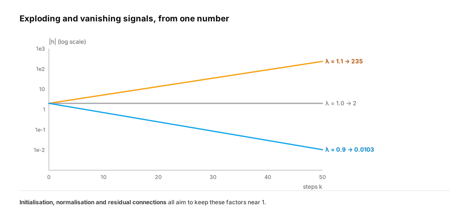
Fifty steps with eigenvalue 0.9 shrink the signal by a factor of about 200; with 1.1 they grow it by over 100. This is why initialization schemes and normalization (D4) aim to keep the relevant eigenvalues (or singular values) near 1.
The checks print True for every eigenpair and for the reconstruction. The recurrence takes |h| from 2 to 1.03e-02 (λ = 0.9) or 2.35e+02 (λ = 1.1).
In production. Deep networks multiply many matrices together, layer after layer, so the same arithmetic governs whether gradients survive. Xavier/Glorot and Kaiming/He initialisation choose weight scales so that typical singular values sit near 1. Residual connections add an identity path, so each block's Jacobian is close to I. Gradient clipping caps the occasional explosion. When a training run's loss suddenly becomes NaN, a growing gradient norm in the logs is usually this story.
Quick check
Why does a plain RNN struggle to learn dependencies 100 steps back, while a transformer with residual connections trains fine at that depth?
Show the answer
B. Backpropagating through 100 steps multiplies by the recurrent Jacobian 100 times, so components with |λ| < 1 vanish (and > 1 explode); residual paths keep an identity term so gradients don't decay geometrically — Repeated multiplication scales each eigen-direction by λ^k. Residual connections (and attention's direct links between distant positions) give gradients short, near-identity routes, avoiding the geometric decay.
4. Power iteration: the dominant eigenvector
The question. How do you find the most important eigenvector of a huge matrix without a full decomposition?
Start from nothing. Multiply any starting vector by A repeatedly and normalize: components along smaller eigenvalues shrink relative to the largest, so the vector converges to the dominant eigenvector. This is power iteration, the idea behind PageRank (the stationary distribution of a random walk on a link graph) and a building block of methods for top-k eigenvectors of large covariance matrices.
import numpy as np

links = {0: [1, 2], 1: [2], 2: [0], 3: [2], 4: [2, 3]}          # page -> pages it links to
n, d = 5, 0.85
M = np.zeros((n, n))
for src, outs in links.items():
    for dst in outs:
        M[dst, src] = 1 / len(outs)                              # column-stochastic transition matrix
G = d * M + (1 - d) / n                                          # teleportation keeps it well behaved
r = np.ones(n) / n
for it in range(100):
    r_new = G @ r
    if np.abs(r_new - r).sum() < 1e-10:
        break
    r = r_new
vals, vecs = np.linalg.eig(G)
dominant = np.real(vecs[:, np.argmax(np.real(vals))]); dominant /= dominant.sum()
print(f"power iteration converged in {it} steps: {np.round(r, 3)}")
print(f"dominant eigenvector (eigenvalue {np.max(np.real(vals)):.2f}):    {np.round(dominant, 3)}")
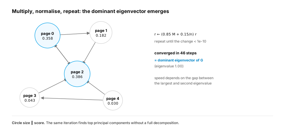
Page 2, which everyone links to, gets the highest score, and power iteration matches the full eigendecomposition. The convergence speed depends on the gap between the largest and second-largest eigenvalue, a recurring theme in numerical methods.
Power iteration converges in 46 steps to [0.358 0.182 0.386 0.043 0.03], identical to the dominant eigenvector (eigenvalue 1.00) from the full decomposition. Page 0 is second only because the highly ranked page 2 links to it: a link from an important page counts for more.
In production. Power iteration and its relatives (Lanczos, randomised SVD) are how "top-k eigenvectors" are computed at scale, for graph ranking, spectral clustering and PCA on huge data, because each step needs only a matrix-vector product, which works on sparse matrices too large to decompose. Optimisers rely on the same idea to estimate the largest eigenvalue of a loss surface's curvature, which bounds the usable learning rate (Optimization).
Quick check
Two input features are almost perfectly correlated. What happens to plain least-squares weights, and why?
Show the answer
C. X^T X is nearly singular (huge condition number), so the weights become large, opposite-signed and unstable under small data changes; ridge regularization fixes the conditioning — Near-dependence makes the smallest eigenvalue of X^T X tiny, so its inverse amplifies noise. Adding λI lifts all eigenvalues by λ and stabilizes the solution.
Check yourself
- Why solve the normal equations with a solver instead of computing (XᵀX)⁻¹?
- What does a rank-deficient feature matrix mean for the learned weights?
- Define eigenvector and eigenvalue, and explain A = QΛQᵀ for symmetric A.
- How do eigenvalues explain exploding and vanishing signals?
- How does power iteration work, and what controls its speed?
- A model's coefficients flip sign between weekly retrains while accuracy stays the same. What's the likely cause and fix?
Answers
- Solvers are faster and more numerically stable; explicit inverses amplify rounding errors, especially for ill-conditioned matrices.
- Infinitely many weight vectors fit equally well (no unique solution); near rank-deficiency makes weights unstable.
- Av = λv: A only scales v by λ. A symmetric matrix decomposes into orthonormal eigenvectors Q and eigenvalues Λ: rotate, scale each axis, rotate back.
- Repeated application scales each eigen-direction by λᵏ, exploding if |λ| > 1 and vanishing if |λ| < 1.
- Repeatedly multiply by A and normalize; the dominant eigenvector takes over. Speed depends on the ratio of the second-largest to largest eigenvalue.
- Nearly collinear features make XᵀX ill-conditioned, so only their combined effect is determined. Remove or combine the duplicates, or add ridge regularisation.
Exercise
Implement deflation: after finding the dominant eigenvector v₁ of a symmetric matrix with power iteration, subtract λ₁v₁v₁ᵀ and run power iteration again to get the second eigenvector. Test on the covariance matrix of 3-D data with a clear main direction, and compare with np.linalg.eigh.
Solution
import numpy as np

rng = np.random.default_rng(3)
data = rng.standard_normal((1000, 3)) @ np.array([[3.0, 0, 0], [1.0, 1.5, 0], [0, 0.5, 0.5]])
C = np.cov(data, rowvar=False)

def power(A, iters=500):
    v = rng.standard_normal(A.shape[0])
    for _ in range(iters):
        v = A @ v; v /= np.linalg.norm(v)
    return v @ A @ v, v

l1, v1 = power(C)
l2, v2 = power(C - l1 * np.outer(v1, v1))
vals, vecs = np.linalg.eigh(C)
print(f"power + deflation: {l1:.3f}, {l2:.3f}   eigh: {vals[-1]:.3f}, {vals[-2]:.3f}")
print("directions match (|cos|):", round(abs(v1 @ vecs[:, -1]), 4), round(abs(v2 @ vecs[:, -2]), 4))
Deflation removes the dominant direction so that power iteration then finds the next one. The values and directions match the full decomposition, which is how top-k eigenvectors of covariance matrices (the next lesson's principal components) can be computed without decomposing the whole matrix.
This unlocks:
- SVD and PCA — the decomposition behind dimensionality reduction, LoRA and embeddings analysis.
- Calculus and Optimization — conditioning shapes how gradient descent behaves.
Sources: Strang, Introduction to Linear Algebra (5th ed.); Trefethen & Bau, Numerical Linear Algebra (1997); Page, Brin et al., The PageRank Citation Ranking (1999); Pascanu, Mikolov & Bengio, On the difficulty of training recurrent neural networks (2013).