You already know: models output probability distributions via softmax, and training minimizes negative log-likelihood (Probability §1, §5); optimizers minimize a loss with gradients (Optimization).
Why this matters for Atlas. "Cross-entropy loss", "perplexity", "KL penalty", "bits per byte" — these words appear in every LLM paper and training dashboard. They're all one idea: how surprised is a model by what actually happens? Information theory makes that precise and explains why compression and prediction are the same problem.
1. Information: surprise in bits
The question. How much "information" does learning one outcome give you?
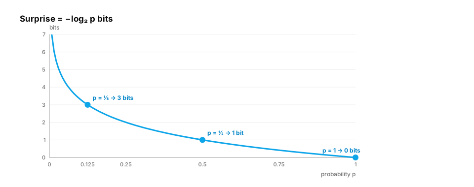
Start from nothing. An unlikely event tells you more than a likely one. Claude Shannon defined the information (surprise) of an outcome with probability p as:
I(x) = −log₂ p(x) bits
- A fair coin flip (p = ½): 1 bit.
- One of 8 equally likely options: 3 bits.
- Something with probability 1: 0 bits — no surprise at all.
Using log₂ measures bits; using the natural log ln measures nats (ML frameworks use nats; divide by ln 2 ≈ 0.693 to convert).
Real-life analogy. "The sun rose today" carries almost no news. "It snowed in the Sahara" is front-page news. Less likely → more information.
Worked example.
import math

for label, p in [("fair coin", 0.5), ("one of 8", 1 / 8), ("50k-word vocab, uniform", 1 / 50_000),
                 ("model says 90%", 0.9), ("model says 1%", 0.01)]:
    print(f"{label:25s} p={p:<8.5g} surprise = {-math.log2(p):6.2f} bits")
Quick check
An event has probability 1/1024. How many bits of information does observing it carry?
Show the answer
C. 10 bits (−log₂ 1/1024) — Information is −log₂ p: rare events are surprising. Each halving of probability adds one bit, and 1/1024 is ten halvings.
2. Entropy: average surprise of a distribution
The question. How unpredictable is a whole distribution — say, the next word in English?
Start from nothing. Entropy is the expected surprise:
H(p) = −Σ p(x) log₂ p(x)
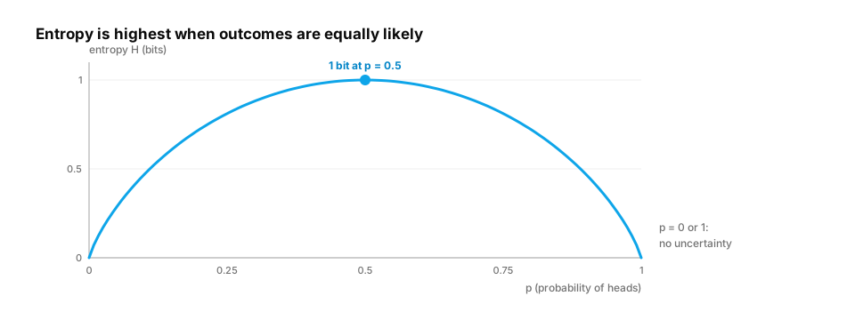
It's highest when every outcome is equally likely (maximum uncertainty) and zero when one outcome is certain. Shannon showed entropy is the minimum average number of bits needed to encode outcomes from that distribution — the limit of lossless compression.
Worked example.
import numpy as np

def entropy_bits(p):
    p = np.asarray(p, dtype=float)
    p = p[p > 0]
    return float(-(p * np.log2(p)).sum())

print(entropy_bits([0.5, 0.5]))            # 1.0
print(entropy_bits([0.99, 0.01]))          # 0.081 — almost certain
print(entropy_bits([0.25] * 4))            # 2.0
print(entropy_bits([0.7, 0.2, 0.05, 0.05]))
In production. The entropy of a model's next-token distribution is a cheap uncertainty signal: high entropy at a factual position ("The capital of Peru is ___") can flag answers that need retrieval or a check.
From production
Two vocabularies are compared by the entropy of their next-token distributions on the same text. Tokenizer B has higher per-token entropy but produces 30% fewer tokens.
Which comparison is fair?
Show the answer
D. Normalise per character or per byte (e.g. bits per byte): per-token numbers depend on how much text each token covers — Bigger tokens carry more text each, so their per-token entropy rises even if the model is equally good. Per-byte (or per-character) metrics make tokenizers comparable.
3. Cross-entropy: surprise when you use the wrong distribution
The question. What exactly is the "cross-entropy loss" on every training dashboard?
Start from nothing. Suppose reality follows distribution p, but your model believes q. If you encode reality using the model's probabilities, your average surprise is the cross-entropy:
H(p, q) = −Σ p(x) log q(x)
For training, p is the data: the actual next token gets probability 1, everything else 0. The sum collapses to one term:
loss = −log q(actual next token)
which is exactly the negative log-likelihood from Probability §5. Training an LLM = making it less surprised by real text, one token at a time. Cross-entropy is never smaller than the true entropy H(p) — the gap is how wrong the model is (section 4).
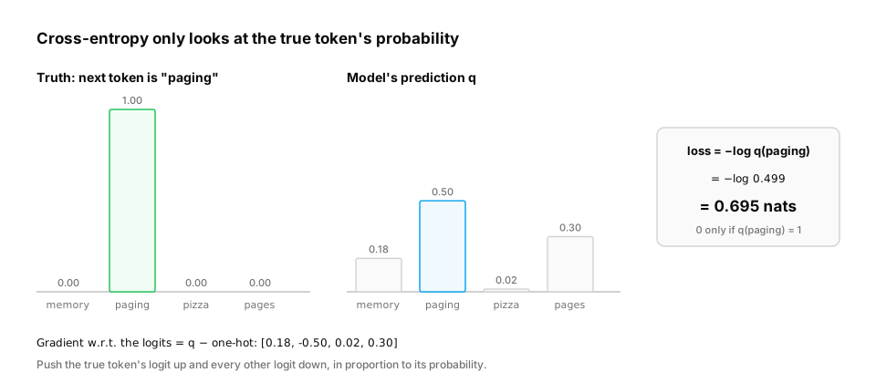
Worked example — the loss for one prediction, and the gradient that makes training easy:
import numpy as np

vocab = ["memory", "paging", "pizza", "pages"]
logits = np.array([1.5, 2.5, -1.0, 2.0])
target = vocab.index("paging")

probs = np.exp(logits - logits.max()); probs /= probs.sum()
loss = -np.log(probs[target])
print("probabilities:", probs.round(3), "loss (nats):", round(float(loss), 3))

# The gradient of cross-entropy w.r.t. the logits is beautifully simple: probs - one_hot
one_hot = np.eye(len(vocab))[target]
print("gradient:", (probs - one_hot).round(3))
That last line is why softmax + cross-entropy is the standard pairing: the gradient is "what you predicted minus what was true", with no vanishing slope even when the model is badly wrong.
From production
A classifier's validation cross-entropy keeps improving, but accuracy has been flat for several epochs.
What can explain this?
Show the answer
B. Cross-entropy also rewards becoming more confident on examples already classified correctly (and less confidently wrong), without changing which class wins, so loss can fall while accuracy stays the same — Cross-entropy depends on the probability of the true class, not just the argmax. Shifting probability mass towards correct answers lowers the loss even when no prediction flips.
4. KL divergence: the gap between two distributions
The question. How do we measure how different a fine-tuned model has become from the original?
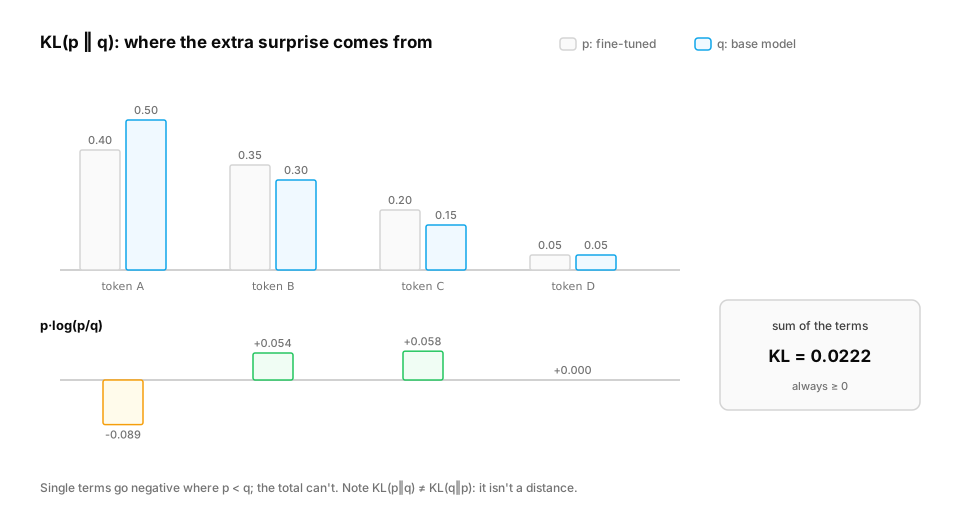
Start from nothing. The Kullback–Leibler divergence is the extra surprise you pay for using q instead of the true p:
D_KL(p ‖ q) = Σ p(x) log (p(x) / q(x)) = H(p, q) − H(p)
Properties:
- Always ≥ 0, and 0 only when
p = q. - Not symmetric:
D_KL(p‖q) ≠ D_KL(q‖p)in general, so it isn't a true distance.
Where it appears in AI:
- RLHF / DPO (D6): a KL penalty keeps the fine-tuned model close to the original, so it doesn't drift into nonsense while chasing reward.
- Distillation: train a small model to minimize KL to a big model's distribution.
- Quantization and serving (D12): compare a quantized model's outputs to the full-precision model's.
Worked example.
import numpy as np

def kl(p, q):
    p, q = np.asarray(p, float), np.asarray(q, float)
    mask = p > 0
    return float((p[mask] * np.log(p[mask] / q[mask])).sum())

base       = np.array([0.50, 0.30, 0.15, 0.05])   # original model
finetuned  = np.array([0.40, 0.35, 0.20, 0.05])   # gentle change
collapsed  = np.array([0.97, 0.01, 0.01, 0.01])   # over-optimized, everything on one answer

print(f"KL(finetuned || base) = {kl(finetuned, base):.4f}")
print(f"KL(collapsed || base) = {kl(collapsed, base):.4f}")
print(f"asymmetry: KL(base || collapsed) = {kl(base, collapsed):.4f}")
Common trap. Computing KL where q(x) = 0 but p(x) > 0 gives infinity. In practice probabilities from softmax are never exactly zero, but quantized or truncated (top-k) distributions can be — add a small epsilon or compare on shared support.
From production
An RLHF run optimises a reward model's score. Without a KL penalty to the reference model, outputs drift into repetitive, oddly phrased text that scores highly.
What does the KL term in the objective do?
Show the answer
C. It penalises the policy for moving far from the reference model's distribution, limiting reward hacking and keeping outputs fluent — D_KL(policy ‖ reference) grows as the policy's token distribution departs from the reference. The penalty trades reward against staying close to sensible language, which mitigates exploiting the reward model's blind spots.
5. Perplexity and bits per byte: reading LLM metrics
The question. A paper reports "perplexity 8.2". Is that good?
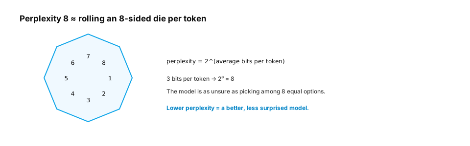
Start from nothing. Perplexity is the exponential of the average cross-entropy (in nats):
PPL = e^{loss}
Intuition: the model is as uncertain as if it were choosing uniformly among PPL options at every step. Lower is better. Perplexity depends on the tokenizer (different tokens, different counts), so comparisons are only fair with the same tokenizer and data. Bits per byte (cross-entropy in bits divided by the number of bytes of text) is tokenizer-independent and lets you compare models with different vocabularies.
Worked example.
import math

token_probs = [0.6, 0.2, 0.9, 0.05, 0.7, 0.4]     # model's probability for each actual token
nll = [-math.log(p) for p in token_probs]
avg = sum(nll) / len(nll)
print(f"average loss {avg:.3f} nats -> perplexity {math.exp(avg):.2f}")

text_bytes = 30                                   # bytes of text those 6 tokens covered
bits = sum(nll) / math.log(2)
print(f"bits per byte = {bits / text_bytes:.3f}")
In production / interviews. Interview question: "Validation loss fell from 2.10 to 2.05 nats. What's the perplexity change, and is it meaningful?" (e^2.10 ≈ 8.17 → e^2.05 ≈ 7.77, about 5% fewer effective choices per token — meaningful at scale, but confirm on downstream evals.)
Quick check
Model A has perplexity 8 and model B perplexity 16 on the same test set and tokenizer. What does that mean?
Show the answer
A. On average A is as uncertain as a uniform choice among 8 tokens and B among 16; A assigns higher probability to the actual text (1 bit per token lower cross-entropy) — Perplexity = 2^(cross-entropy in bits). Going from 16 to 8 halves the effective number of choices, i.e. one bit less surprise per token. Comparisons only hold on the same data and tokenizer.
6. Compression = prediction
The question. Why do people say a language model "is" a compressor?
Start from nothing. Shannon's coding theorem says an event of probability p can be encoded in about −log₂ p bits (arithmetic coding gets very close). So a model that assigns higher probability to real text can compress that text into fewer bits. Better prediction → better compression, exactly. Minimizing cross-entropy during training is minimizing the compressed size of the training data.
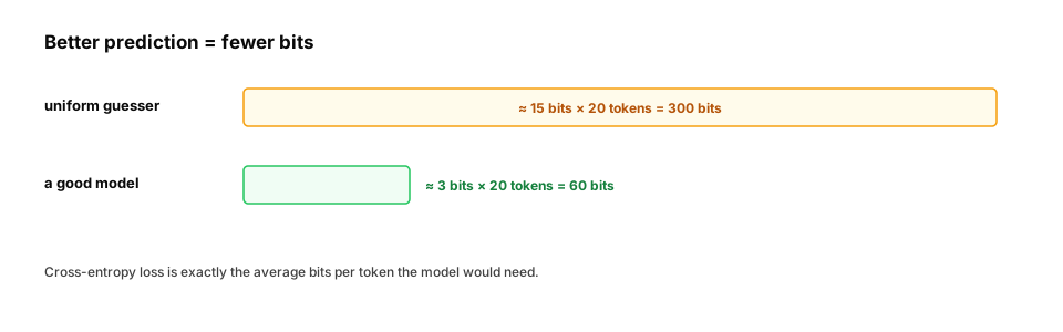
Worked example — the bit cost of a message under two models:
import math

message = "the gpu ran out of memory".split()
uniform = {w: 1 / 50_000 for w in message}                      # knows nothing
good_lm = {"the": 0.05, "gpu": 0.002, "ran": 0.1, "out": 0.6, "of": 0.9, "memory": 0.4}

for name, model in [("uniform guess", uniform), ("good language model", good_lm)]:
    bits = sum(-math.log2(model[w]) for w in message)
    print(f"{name:20s}: {bits:6.1f} bits for {len(message)} words")
Quick check
A model's validation cross-entropy is 2.0 nats per token. What is its perplexity?
Show the answer
C. e² ≈ 7.4: on average the model is as uncertain as choosing among about 7 equally likely tokens — Perplexity is the exponential of the average cross-entropy (in nats).
Check yourself
- Recall: What is the entropy of a fair 4-sided die?
- Apply: The model gives the correct token probability 0.25. What's the loss in nats and in bits?
- Predict: Is
D_KL(p‖q)equal toD_KL(q‖p)? - Apply: Why compare models with different tokenizers using bits per byte rather than per-token loss?
- Explain: Why can validation loss keep falling while accuracy stays flat?
Answers
- 2 bits.
−ln 0.25 ≈ 1.386nats =−log₂ 0.25 = 2bits.- Not in general — KL divergence is asymmetric.
- Per-token numbers depend on how much text a token covers; normalising by bytes measures prediction quality on the same underlying text.
- Cross-entropy rewards putting more probability on the correct class even when the argmax doesn't change, so confidence improves without flipping predictions.
Exercise
Write distill_loss(student_logits, teacher_logits, temperature) that returns T² · KL(teacher_soft ‖ student_soft) (the standard knowledge-distillation loss), and show that it is 0 when the logits match and grows as they diverge. Then compute the perplexity of a uniform model over a 50,000-token vocabulary.
Solution
import numpy as np

def softmax(z):
    z = np.asarray(z, float); e = np.exp(z - z.max()); return e / e.sum()

def distill_loss(student_logits, teacher_logits, T=2.0):
    p = softmax(np.asarray(teacher_logits) / T)
    q = softmax(np.asarray(student_logits) / T)
    return float(T ** 2 * (p * np.log(p / q)).sum())

teacher = [3.0, 1.0, 0.2]
for student in ([3.0, 1.0, 0.2], [2.5, 1.2, 0.3], [0.0, 3.0, 0.0]):
    print(student, round(distill_loss(student, teacher), 4))

print("uniform 50k-vocab perplexity:", round(float(np.exp(-np.log(1 / 50_000))), 1))   # 50000.0
This unlocks:
- D3 Supervised learning — logistic regression's loss is cross-entropy.
- D5 LLM pretraining — next-token cross-entropy, perplexity and scaling laws.
- D6 Preference optimization — the KL penalty in RLHF and DPO.
- D12 Quantization — measuring how much a compressed model drifts (KL to the original).
Sources: Shannon, A Mathematical Theory of Communication (1948); Cover & Thomas, Elements of Information Theory; MacKay, Information Theory, Inference, and Learning Algorithms; Hinton et al., Distilling the Knowledge in a Neural Network (2015); Delétang et al., Language Modeling Is Compression (2024).