You already know: regression and classification (Supervised learning), clustering and anomaly detection (Unsupervised learning), and similarity with dot products (D2 Linear algebra §2).
Why this matters for Atlas. The hardest step in applied ML is often not the model — it's deciding what kind of problem you're solving. "Help students learn faster" could be classification (will they quit?), ranking (which lesson first?), recommendation (what's next for this student?), or forecasting (how many GPUs tomorrow?). Each family has its own data shape, models and metrics. Many LLM systems — retrieval-augmented generation, routing, reranking — are these classic families wearing new clothes.
1. Framing: from a product question to an ML family
The question. How do you turn a vague goal into a problem a model can solve?
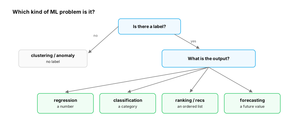
Start from nothing. Ask three things: What is the output? What data do we have about the right answer? How will the prediction be used?
| Product question | Output | Family | Typical first model |
|---|---|---|---|
| Will this student quit this week? | yes / no + probability | Classification | Logistic regression, boosted trees |
| How many tokens will this answer use? | a number | Regression | Linear model, boosted trees |
| Which 10 lessons best match this search? | an ordered list | Ranking / retrieval | BM25, then learning to rank |
| What should this student study next? | personalized list | Recommendation | Popularity baseline, matrix factorization |
| How many requests will hit us at 9 a.m.? | future values over time | Forecasting | Seasonal naive, gradient boosting on lags |
| What topics do questions fall into? | groups | Clustering | k-means on embeddings |
| Is this API call abuse? | unusual / normal | Anomaly detection | Isolation Forest, thresholds |
Common trap. Solving a ranking problem as classification. "Is this lesson relevant? yes/no" ignores that what users see is the order — and the right metric for order is different (lesson 5).
2. Retrieval and ranking: finding the best items fast
The question. A student types "why does my GPU run out of memory". How does Atlas pick the 10 best lessons out of thousands?
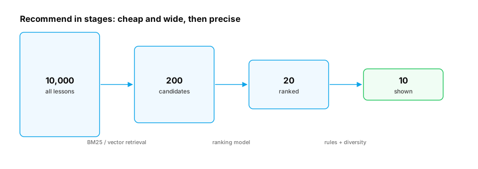
Start from nothing. Ranking systems usually work in stages, because the best scorer is too slow to run on everything:
- Retrieval — cheaply narrow millions of items to hundreds of candidates. Classic method: BM25, a keyword score that rewards query words that are rare across documents (high inverse document frequency) and appear often in this document — with diminishing returns and a correction for long documents. Modern systems add vector retrieval with embeddings (D8).
- Ranking — score each candidate with a richer model (more features, or a cross-encoder) and sort.
- Re-ranking and rules — business logic: diversity, freshness, "don't show locked lessons to free users".
Learning to rank trains the ranking model from feedback (clicks, completions): pointwise (predict relevance of each item), pairwise (predict which of two items is better), or listwise (optimize the whole list's metric).
Real-life analogy. Hiring: a quick CV keyword scan (retrieval), then interviews for the shortlist (ranking), then a final check on team fit and budget (rules).
Worked example — BM25 from scratch:
import math
from collections import Counter

docs = {
    "gpu-memory":   "gpu memory runs out when the kv cache and activations exceed gpu memory capacity",
    "paging":       "virtual memory paging maps pages of memory to physical frames",
    "tcp":          "tcp makes delivery reliable with retransmission and ordering",
    "quantization": "quantization stores weights in fewer bits to save gpu memory",
}
tokenized = {k: v.split() for k, v in docs.items()}
N = len(docs)
avgdl = sum(len(t) for t in tokenized.values()) / N
df = Counter(word for toks in tokenized.values() for word in set(toks))

def bm25(query, doc_tokens, k1=1.5, b=0.75):
    tf = Counter(doc_tokens)
    score = 0.0
    for word in query.split():
        if word not in tf:
            continue
        idf = math.log(1 + (N - df[word] + 0.5) / (df[word] + 0.5))
        norm = tf[word] * (k1 + 1) / (tf[word] + k1 * (1 - b + b * len(doc_tokens) / avgdl))
        score += idf * norm
    return score

query = "why does my gpu run out of memory"
for name in sorted(docs, key=lambda d: -bm25(query, tokenized[d])):
    print(f"{bm25(query, tokenized[name]):.3f}  {name}")
Output: gpu-memory 2.402, paging 1.748, quantization 1.073, tcp 0.000.
Notice the weaknesses. "paging" — a lesson about CPU virtual memory — beats "quantization", a lesson that really is about saving GPU memory, simply because it repeats the word "memory" three times. "run" doesn't match "runs", and nothing understands meaning. That's why production search combines BM25 with embeddings (hybrid retrieval, D8) and reranks the candidates.
3. Recommendation: personalizing for each user
The question. Two students both finished "Python internals". Should they get the same next lesson?
Start from nothing. Recommendation predicts what this user will value from what similar users valued:
- Popularity baseline — recommend what's most completed. Hard to beat for new users.
- Content-based — recommend items similar to ones the user liked (item features / embeddings).
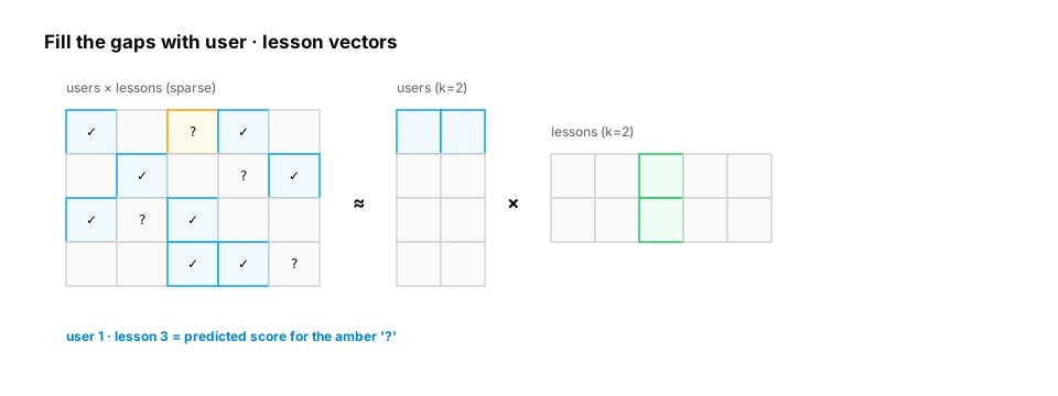
- Collaborative filtering — learn from the user × item interaction matrix alone. Matrix factorization gives every user and item a small vector so that
user · item ≈ affinity; missing entries in the matrix become predictions.
Practical issues: cold start (new users/items have no history — fall back to popularity or content), feedback loops (you only learn about items you showed), and the same multi-stage retrieve → rank → rerank pipeline as search.
Worked example — matrix factorization by gradient descent:
import numpy as np

rng = np.random.default_rng(0)
n_users, n_lessons, k = 40, 12, 3
true_u, true_v = rng.normal(size=(n_users, k)), rng.normal(size=(n_lessons, k))
ratings = true_u @ true_v.T                                   # hidden "true" affinities
observed = rng.random(ratings.shape) < 0.3                    # we only see 30% of pairs

U = 0.1 * rng.normal(size=(n_users, k))
V = 0.1 * rng.normal(size=(n_lessons, k))
lr, reg = 0.05, 0.01
for epoch in range(400):
    err = np.where(observed, U @ V.T - ratings, 0.0)          # error only on observed cells
    U -= lr * (err @ V + reg * U)
    V -= lr * (err.T @ U + reg * V)

pred = U @ V.T
rmse_seen = np.sqrt(((pred - ratings)[observed] ** 2).mean())
rmse_unseen = np.sqrt(((pred - ratings)[~observed] ** 2).mean())
baseline = np.sqrt(((ratings[observed].mean() - ratings)[~observed] ** 2).mean())
print(f"RMSE on seen pairs {rmse_seen:.3f} | unseen pairs {rmse_unseen:.3f} | predict-the-average {baseline:.3f}")
Output: RMSE ≈ 0.06 on seen pairs, ≈ 0.95 on unseen pairs, ≈ 1.60 for predicting the average. The model predicts pairs it never saw much better than the average — that's personalization. The big gap between seen and unseen error is overfitting to the 30% of observed cells; stronger regularization (reg), fewer factors or more data narrow it, and the unseen error is the number to report.
4. Forecasting: predicting the future of a time series
The question. How many requests per hour will Atlas get tomorrow, so we can provision GPUs?
Start from nothing. A time series is a sequence of values over time. Patterns to capture: trend (slowly growing), seasonality (daily and weekly cycles), and noise. Two rules that trip people up:
- Always beat a naive baseline first. "Same hour yesterday" (seasonal naive) is often surprisingly strong.
- Split by time, never randomly. Train on the past, test on the future — a random split leaks future information into training.
A practical recipe: build lag features (value 1 hour ago, 24 hours ago, 168 hours ago), calendar features (hour of day, weekday), and fit a regression model.
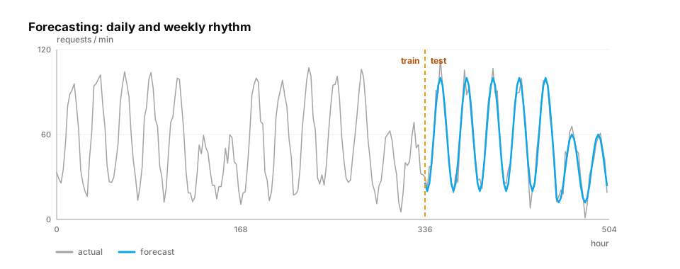
Worked example.
import numpy as np
from sklearn.ensemble import HistGradientBoostingRegressor

rng = np.random.default_rng(0)
hours = np.arange(24 * 7 * 8)                                   # 8 weeks hourly
hour_of_day, day_of_week = hours % 24, (hours // 24) % 7
traffic = (200 + 0.3 * hours                                    # trend
           + 150 * np.sin(2 * np.pi * (hour_of_day - 8) / 24)   # daily cycle
           - 80 * (day_of_week >= 5)                            # quieter weekends
           + rng.normal(0, 25, hours.size))

def features(t):
    return np.column_stack([traffic[t - 1], traffic[t - 24], traffic[t - 168], hour_of_day[t], day_of_week[t]])

t_all = np.arange(168, hours.size)
split = hours.size - 24 * 7                                     # last week is the test set
train_t, test_t = t_all[t_all < split], t_all[t_all >= split]

model = HistGradientBoostingRegressor(random_state=0).fit(features(train_t), traffic[train_t])
mae_model = np.abs(model.predict(features(test_t)) - traffic[test_t]).mean()
mae_naive = np.abs(traffic[test_t - 24] - traffic[test_t]).mean()   # "same hour yesterday"
print(f"seasonal naive MAE {mae_naive:.1f} | gradient boosting MAE {mae_model:.1f}")
(This model predicts one hour ahead using the previous hour; forecasting a full day ahead needs features available that far in advance — exactly the leakage question of the next lesson.)
5. Classic case studies, and their LLM-era versions
The question. Where do these families show up together in real systems?
| Case | Classic pipeline | The same pattern in LLM systems |
|---|---|---|
| Fraud detection | Features from transactions → classifier → risk score → threshold tuned to the cost of misses vs false alarms → drift monitoring | Abuse / jailbreak detection on LLM APIs (D19) |
| Product recommendation | Candidate retrieval → ranking model → reranking + business rules; cold-start fallbacks; feedback loops | Choosing which documents or tools to give an agent (D8, D9) |
| Search ranking | BM25 + vector retrieval → learning to rank → evaluation with NDCG | Retrieval-augmented generation: retrieve, rerank, then generate (D8) |
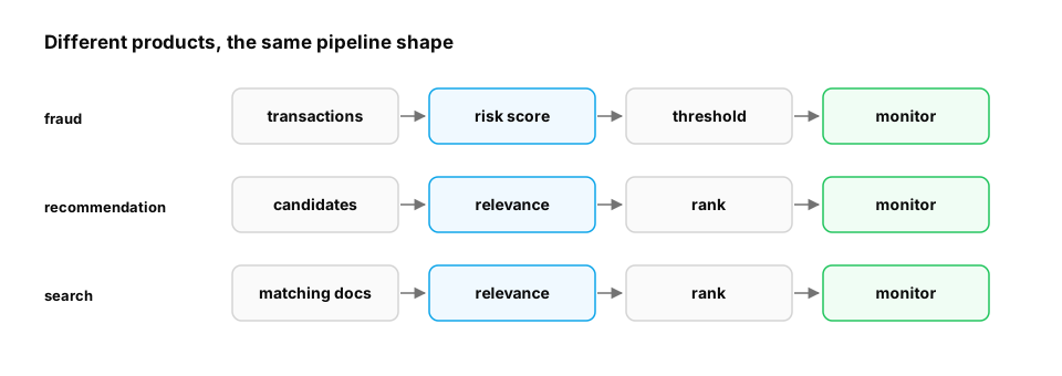
Worked example — choosing a fraud threshold by cost, not accuracy:
import numpy as np

rng = np.random.default_rng(5)
n = 20_000
is_fraud = rng.random(n) < 0.01
score = np.clip(rng.normal(np.where(is_fraud, 0.7, 0.25), 0.15), 0, 1)   # model's risk score

COST_MISSED_FRAUD, COST_FALSE_ALARM = 500, 5        # rupees: a chargeback vs a manual review
best = None
for threshold in np.linspace(0.1, 0.9, 81):
    flagged = score >= threshold
    cost = COST_MISSED_FRAUD * (is_fraud & ~flagged).sum() + COST_FALSE_ALARM * (~is_fraud & flagged).sum()
    if best is None or cost < best[1]:
        best = (threshold, cost, flagged.mean())
print(f"best threshold {best[0]:.2f}: total cost ₹{best[1]:,}, flags {best[2]:.1%} of transactions")
print("accuracy at threshold 0.5:", round(((score >= 0.5) == is_fraud).mean(), 4))   # ~0.95
print("accuracy of 'never fraud':", round((~is_fraud).mean(), 4))                   # ~0.99 — and catches nothing
# Accuracy rewards ignoring a rare class. Optimize the business cost (or precision/recall) instead.
Quick check
A team frames 'which lessons should a student see' as binary classification of every lesson, independently. What's the better framing?
Show the answer
C. A ranking problem: retrieve candidates, then order them for each student, evaluated with ranking metrics like NDCG or recall@k — The product shows an ordered short list; ranking objectives and metrics match that, independent classification doesn't.
Check yourself
- Recall: Name the three typical stages of a search or recommendation system.
- Apply: You're predicting next week's GPU demand. How should you split train and test data?
- Predict: In the BM25 example, why does "quantization" score above "tcp" for the GPU-memory query?
Answers
- Candidate retrieval → ranking → re-ranking with business rules.
- By time: train on earlier weeks, test on later weeks — never a random split.
- It contains "gpu" and "memory", both query words; "tcp" shares none.
Exercise
Build a two-stage lesson recommender: stage 1 retrieves the 5 lessons with the highest BM25 score for a student's question; stage 2 re-ranks them with 0.7 × normalized BM25 + 0.3 × predicted affinity from a matrix-factorization model, and finally removes lessons the student has already completed.
Solution sketch
import math
from collections import Counter
import numpy as np

lessons = ["gpu memory kv cache", "virtual memory paging", "tcp reliable delivery",
           "quantization fewer bits gpu memory", "attention softmax queries keys", "batching gpu throughput"]
toks = [l.split() for l in lessons]
N, avgdl = len(toks), sum(map(len, toks)) / len(toks)
df = Counter(w for t in toks for w in set(t))

def bm25(q, t, k1=1.5, b=0.75):
    tf = Counter(t)
    return sum(math.log(1 + (N - df[w] + .5) / (df[w] + .5)) * tf[w] * (k1 + 1)
               / (tf[w] + k1 * (1 - b + b * len(t) / avgdl)) for w in q.split() if w in tf)

rng = np.random.default_rng(0)
affinity = rng.uniform(0, 1, N)                  # stand-in for this student's MF predictions
completed = {1}                                  # already finished "virtual memory paging"

question = "gpu memory problems"
scores = np.array([bm25(question, t) for t in toks])
candidates = np.array([i for i in np.argsort(-scores) if scores[i] > 0][:5])   # drop zero-match lessons
bm = scores[candidates] / (scores[candidates].max() or 1)
final = 0.7 * bm + 0.3 * affinity[candidates]
ranked = [lessons[i] for i in candidates[np.argsort(-final)] if i not in completed]
print(ranked)
This unlocks:
- Feature engineering — the inputs every family above depends on.
- ML evaluation — the right metric for each family (NDCG for ranking, MAE for forecasts, cost for fraud).
- D8 Retrieval fundamentals & advanced RAG — BM25 + vectors + reranking.
Sources: Robertson & Zaragoza, The Probabilistic Relevance Framework: BM25 and Beyond (2009); Koren, Bell & Volinsky, Matrix Factorization Techniques for Recommender Systems (2009); Hyndman & Athanasopoulos, Forecasting: Principles and Practice; Covington et al., Deep Neural Networks for YouTube Recommendations (2016).