
You already know: confidence intervals and paired bootstrap comparisons (D2 Probability §6), cross-entropy (D2 Information theory §3), leakage and time-based splits (Feature engineering §5), and why accuracy misleads on rare classes (ML problem families §5).
Why this matters for Atlas. A metric is a promise about the future: "this model will behave like this on new students". Every later evaluation topic — LLM evals (D10), RAG evals (D8), monitoring (D11) — is built on the ideas here: honest splits, the right metric for the decision, calibrated probabilities, and offline numbers that actually predict online results.
1. Splits: train, validation, test — and cross-validation
The question. Where should the numbers we report come from?
Start from nothing.
- Training set — the model learns from it.
- Validation set — we use it to choose models and hyperparameters. Because we make decisions with it, it gets slightly "used up".
- Test set — touched once, at the end, to estimate real-world performance.
With limited data, k-fold cross-validation rotates the validation role: split into k folds, train on k−1, validate on the remaining one, repeat k times, average. Choose the split shape to match how the model will be used:
- Stratified — keeps the class ratio equal in every fold (important for rare classes).
- Grouped — all rows of one user stay in the same fold (otherwise the model memorizes users).
- Time-based — always validate on later data than you trained on.
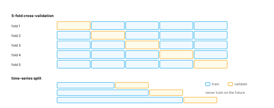
Worked example — a grouped split exposes memorization:
import numpy as np
from sklearn.ensemble import RandomForestClassifier
from sklearn.model_selection import GroupKFold, KFold, cross_val_score

rng = np.random.default_rng(0)
users, rows_per_user = 100, 20
user_id = np.repeat(np.arange(users), rows_per_user)
user_trait = rng.normal(size=users)[user_id]             # each user has a stable quirk...
X = np.column_stack([user_trait + 0.01 * rng.normal(size=user_id.size), rng.normal(size=(user_id.size, 3))])
y = rng.random(users)[user_id] < 0.5                     # ...and a label unrelated to any generalizable pattern

rf = RandomForestClassifier(n_estimators=100, random_state=0)
print("random K-fold :", cross_val_score(rf, X, y, cv=KFold(5, shuffle=True, random_state=0)).mean().round(3))
print("grouped K-fold:", cross_val_score(rf, X, y, cv=GroupKFold(5), groups=user_id).mean().round(3))
Output: ≈0.76 with random folds, ≈0.57 with grouped folds. With a random split, the forest recognizes each user's quirk and "predicts" their label from their other rows; with a grouped split it drops to about what always guessing the most common label would score — the honest answer for brand-new users.
2. The confusion matrix, precision and recall
The question. "92% accurate" — at what, exactly?
Start from nothing. For a yes/no classifier, count the four outcomes:
| Predicted yes | Predicted no | |
|---|---|---|
| Actually yes | True positive (TP) | False negative (FN) |
| Actually no | False positive (FP) | True negative (TN) |
- Precision
TP / (TP + FP)— of everything we flagged, how much was right? - Recall
TP / (TP + FN)— of everything we should have flagged, how much did we catch? - F1 — their harmonic mean,
2PR / (P + R): high only when both are.
Raising the threshold usually trades recall for precision. Which matters more depends on the cost of each error.
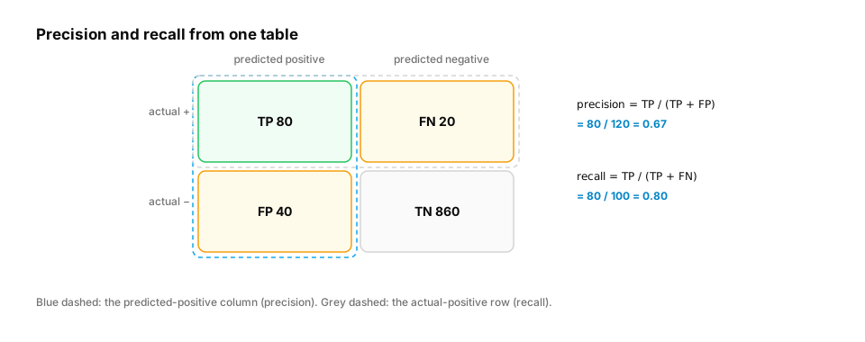
Real-life analogy. A fishing net: precision is "how much of the catch is fish (not boots)"; recall is "how many of the lake's fish did we catch".
Worked example.
import numpy as np
from sklearn.metrics import confusion_matrix, f1_score, precision_score, recall_score

rng = np.random.default_rng(1)
truth = rng.random(5000) < 0.05                                       # 5% of students will quit
score = np.clip(rng.normal(np.where(truth, 0.65, 0.3), 0.15), 0, 1)

for threshold in [0.3, 0.5, 0.7]:
    pred = score >= threshold
    tn, fp, fn, tp = confusion_matrix(truth, pred).ravel()
    print(f"threshold {threshold}: TP={tp:3d} FP={fp:4d} FN={fn:3d} | "
          f"precision {precision_score(truth, pred):.2f} recall {recall_score(truth, pred):.2f} "
          f"F1 {f1_score(truth, pred):.2f} accuracy {(pred == truth).mean():.2f}")
3. ROC-AUC and PR-AUC: judging the score, not one threshold
The question. How do we compare two models before picking a threshold?
Start from nothing. Sweep every threshold and plot:
- ROC curve — recall (true-positive rate) vs false-positive rate. ROC-AUC is the area under it; equivalently, the probability that a random positive gets a higher score than a random negative. 0.5 = random, 1.0 = perfect ranking.
- Precision–recall curve — precision vs recall. PR-AUC (average precision) focuses on the positive class, so it's much more informative when positives are rare: ROC-AUC can look excellent while precision is terrible, because the huge number of negatives keeps the false-positive rate small.
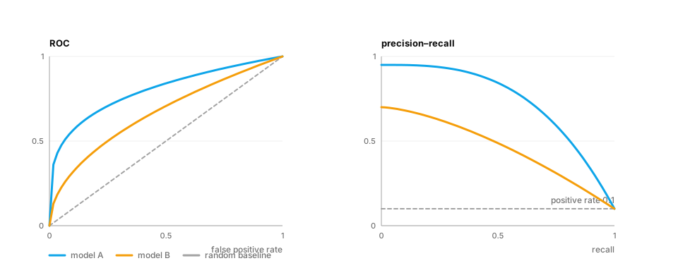
Worked example — the same model on balanced vs rare-positive data:
import numpy as np
from sklearn.metrics import average_precision_score, roc_auc_score

rng = np.random.default_rng(2)
for positive_rate in [0.5, 0.01]:
    truth = rng.random(100_000) < positive_rate
    score = rng.normal(np.where(truth, 1.5, 0.0), 1.0)                # same separation both times
    print(f"positive rate {positive_rate:>4}: ROC-AUC {roc_auc_score(truth, score):.3f}  "
          f"PR-AUC {average_precision_score(truth, score):.3f}  (random PR baseline = {positive_rate})")
ROC-AUC is identical; PR-AUC collapses — because at 1% positives, most flags are false alarms.
4. Calibration and log loss: are the probabilities honest?
The question. The model says "70% likely to quit". Do 70% of such students actually quit?
Start from nothing. A model is calibrated if its predicted probabilities match observed frequencies. Ranking metrics (AUC) ignore calibration entirely — a model can rank perfectly and still say 0.99 when the truth is 0.6. Calibration matters whenever the probability is used as a number: expected cost, risk scores, deciding when an LLM should abstain.
How to measure:
- Reliability diagram — bucket predictions (0–0.1, 0.1–0.2, …) and plot the mean predicted probability vs the observed positive rate; a calibrated model sits on the diagonal.
- Expected calibration error (ECE) — the weighted average gap between those two numbers.
- Log loss (cross-entropy) and Brier score (mean squared error of probabilities) — reward both ranking and calibration.
Fixes: Platt scaling (fit a logistic curve to the scores) or isotonic regression, fitted on validation data.
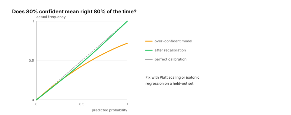
Worked example.
import numpy as np
from sklearn.calibration import CalibratedClassifierCV
from sklearn.datasets import make_classification
from sklearn.metrics import brier_score_loss, log_loss
from sklearn.model_selection import train_test_split
from sklearn.naive_bayes import GaussianNB

X, y = make_classification(n_samples=6000, n_features=20, n_informative=6, n_redundant=10, random_state=0)
X_tr, X_te, y_tr, y_te = train_test_split(X, y, test_size=0.5, random_state=0)

def ece(y_true, p, bins=10):
    edges = np.linspace(0, 1, bins + 1)
    idx = np.clip(np.digitize(p, edges) - 1, 0, bins - 1)
    return sum((idx == b).mean() * abs(p[idx == b].mean() - y_true[idx == b].mean())
               for b in range(bins) if (idx == b).any())

raw = GaussianNB().fit(X_tr, y_tr)                        # naive Bayes is famously over-confident
cal = CalibratedClassifierCV(GaussianNB(), method="isotonic", cv=5).fit(X_tr, y_tr)
for name, m in [("raw naive Bayes", raw), ("isotonic-calibrated", cal)]:
    p = m.predict_proba(X_te)[:, 1]
    print(f"{name:20s} ECE {ece(y_te, p):.3f}  log loss {log_loss(y_te, p):.3f}  Brier {brier_score_loss(y_te, p):.3f}")
5. Ranking metrics: MRR, MAP and NDCG
The question. Search returns 10 lessons. How do we score the list?
Start from nothing. Ranking metrics reward putting relevant items near the top:
- Precision@k / Recall@k — share of the top k that are relevant / share of all relevant items found in the top k.
- MRR (mean reciprocal rank) —
1 / rank of the first relevant item, averaged over queries. Good when one right answer is enough. - MAP (mean average precision) — averages precision at each position where a relevant item appears.
- NDCG@k — handles graded relevance (perfect / good / okay): each item's gain is discounted by
log₂(position + 1), and the total is divided by the best possible ordering's score, giving 0–1.
These are the core metrics for retrieval and RAG (D8).
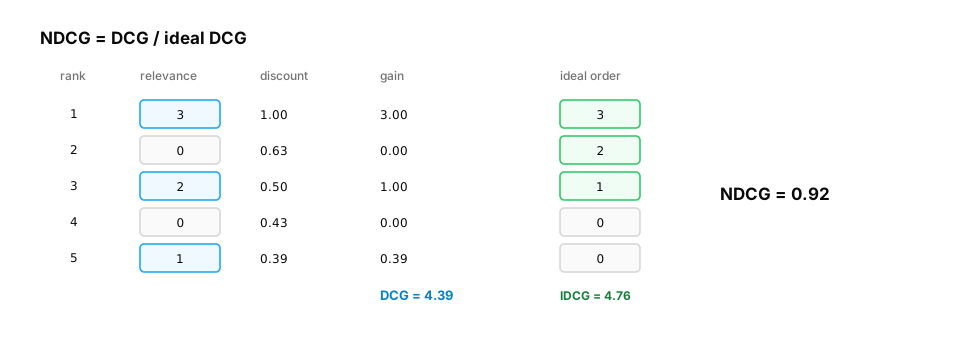
Worked example — implemented from the definitions, checked against scikit-learn:
import numpy as np
from sklearn.metrics import ndcg_score

def dcg(grades):
    grades = np.asarray(grades, float)
    return float((grades / np.log2(np.arange(2, grades.size + 2))).sum())

def ndcg(grades, k=None):
    grades = np.asarray(grades, float)[:k]
    ideal = np.sort(np.asarray(grades, float))[::-1]
    return dcg(grades) / dcg(ideal) if dcg(ideal) > 0 else 0.0

def reciprocal_rank(relevant_flags):
    hits = np.flatnonzero(relevant_flags)
    return 1.0 / (hits[0] + 1) if hits.size else 0.0

ranking = [3, 0, 2, 0, 1]                    # relevance grades of results in the order shown
print("NDCG (ours)   :", round(ndcg(ranking), 4))
print("NDCG (sklearn):", round(ndcg_score([ranking], [[5, 4, 3, 2, 1]]), 4))
print("MRR for [no, no, yes, yes]:", reciprocal_rank([0, 0, 1, 1]))     # first hit at rank 3 -> 1/3
6. Offline vs online: does the metric predict reality?
The question. Model B beats model A offline. Will students actually learn more?
Start from nothing. Offline metrics are measured on historical data; online metrics are what the product cares about (lessons completed, retention, revenue, latency, cost) measured on live traffic. They can disagree because of distribution shift, feedback loops (users only clicked what the old model showed), or a metric that doesn't capture what users value. So:
- Choose offline metrics that correlate with the online goal (and check that they do).
- Confirm with an online A/B test: random split of users, pre-registered metric and duration, a confidence interval on the difference (D2 Probability §6).
- Track guardrail metrics (latency, cost, complaint rate) so a "win" doesn't break something else.
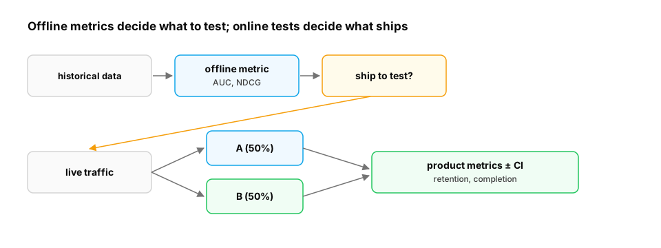
Worked example — a minimal A/B readout with a guardrail:
import numpy as np

rng = np.random.default_rng(4)
n = 8000
group_b = rng.random(n) < 0.5
completed = rng.random(n) < np.where(group_b, 0.315, 0.30)             # primary metric
latency = rng.normal(np.where(group_b, 940, 900), 120)                 # guardrail: ms

def diff_ci(metric_a, metric_b, n_boot=4000):
    boots = [rng.choice(metric_b, metric_b.size).mean() - rng.choice(metric_a, metric_a.size).mean()
             for _ in range(n_boot)]
    return metric_b.mean() - metric_a.mean(), np.percentile(boots, [2.5, 97.5])

for name, m in [("completion rate", completed.astype(float)), ("latency ms", latency)]:
    d, (lo, hi) = diff_ci(m[~group_b], m[group_b])
    print(f"{name:16s} B − A = {d:+.4f}  95% CI [{lo:+.4f}, {hi:+.4f}]")
Output: completion +1.5 points, 95% CI [−0.4, +3.6]; latency +44 ms, 95% CI [+39, +50]. Read it as a decision: the completion gain is not yet distinguishable from zero, while the latency cost is clearly real. Don't ship on this evidence — run longer (or with more users) or reduce B's latency first.
Quick check
A fraud classifier has ROC-AUC 0.96 on data with 0.3% fraud. Why should you also look at the PR curve?
Show the answer
C. With extreme imbalance, a high ROC-AUC can coexist with low precision at useful thresholds; PR curves show precision directly — False-positive rate is computed over a huge negative class, hiding many false alarms; precision exposes them.
Check yourself
- Recall: Precision is TP divided by what?
- Apply: 0.5% of transactions are fraud. Which curve do you show the risk team, ROC or PR?
- Predict: Can a model have ROC-AUC 0.95 and still be badly calibrated?
Answers
- TP + FP — everything predicted positive.
- PR (precision–recall): with rare positives it shows how many flags will be false alarms.
- Yes — AUC only depends on the ordering of scores, not their values.
Exercise
For the "will this student quit?" model, write evaluate(y_true, p, cost_fn, cost_fp) that reports ROC-AUC, PR-AUC, ECE, the cost-minimizing threshold and precision/recall at that threshold. Use a grouped split by student, and recalibrate with isotonic regression on validation data before choosing the threshold.
Solution sketch
import numpy as np
from sklearn.isotonic import IsotonicRegression
from sklearn.linear_model import LogisticRegression
from sklearn.metrics import average_precision_score, precision_score, recall_score, roc_auc_score
from sklearn.model_selection import GroupShuffleSplit

rng = np.random.default_rng(0)
students, per = 600, 10
gid = np.repeat(np.arange(students), per)
X = np.column_stack([rng.normal(size=gid.size) + rng.normal(size=students)[gid], rng.normal(size=gid.size)])
y = rng.random(gid.size) < 1 / (1 + np.exp(-(2.5 * X[:, 0] - 3)))

def ece(t, p, b=10):
    idx = np.clip((p * b).astype(int), 0, b - 1)
    return sum((idx == i).mean() * abs(p[idx == i].mean() - t[idx == i].mean()) for i in range(b) if (idx == i).any())

def evaluate(t, p, cost_fn=50, cost_fp=1):
    ths = np.linspace(0.01, 0.99, 99)
    costs = [cost_fn * (t & (p < th)).sum() + cost_fp * (~t & (p >= th)).sum() for th in ths]
    th = ths[int(np.argmin(costs))]
    pred = p >= th
    return dict(roc=round(roc_auc_score(t, p), 3), pr=round(average_precision_score(t, p), 3),
                ece=round(ece(t, p), 3), threshold=round(th, 2),
                precision=round(precision_score(t, pred), 2), recall=round(recall_score(t, pred), 2))

train_idx, rest = next(GroupShuffleSplit(1, test_size=0.4, random_state=0).split(X, y, gid))
val_idx, test_idx = rest[: len(rest) // 2], rest[len(rest) // 2:]
clf = LogisticRegression(class_weight="balanced").fit(X[train_idx], y[train_idx])   # balanced -> miscalibrated
iso = IsotonicRegression(out_of_bounds="clip").fit(clf.predict_proba(X[val_idx])[:, 1], y[val_idx])

p_raw = clf.predict_proba(X[test_idx])[:, 1]
print("raw       :", evaluate(y[test_idx], p_raw))
print("calibrated:", evaluate(y[test_idx], iso.predict(p_raw)))
This unlocks:
- D4 Neural network fundamentals — the same splits and metrics for deep models.
- D10 Evaluation foundations — evaluating LLMs and agents, where "the label" is fuzzy.
- D8 RAG evaluation — NDCG, MRR and recall@k for retrieval.
- D11 Model monitoring — tracking these metrics after deployment.
Sources: scikit-learn user guide — model evaluation, cross-validation iterators, probability calibration; Saito & Rehmsmeier, The Precision-Recall Plot Is More Informative than the ROC Plot… (2015); Guo et al., On Calibration of Modern Neural Networks (2017); Järvelin & Kekäläinen, Cumulated gain-based evaluation of IR techniques (2002); Kohavi, Tang & Xu, Trustworthy Online Controlled Experiments.