
You already know: models consume numeric feature matrices X (Supervised learning §1); PCA can compress features (Unsupervised learning §4); time series need lag features and time-based splits (ML problem families §4).
Why this matters for Atlas. Real data arrives as logs: some fields missing, plan names as text, timestamps, IDs. A model only sees numbers. How you convert raw data into features often matters more than the choice of model — and doing it carelessly creates the two most expensive bugs in applied ML: data leakage (the model secretly sees the answer) and training-serving skew (features computed differently in production).
1. Missing values
The question. 15% of students have no "minutes per lesson" recorded. Drop them? Fill them in?
Start from nothing. Options, from simplest:
- Drop rows — only if few are missing at random; otherwise you bias the data.
- Impute — fill with the median (robust to outliers), the mean, the most frequent category, or a model's prediction.
- Add a "was missing" indicator — missingness itself is often informative ("no time recorded" may mean the student never opened the lesson).
Crucially, the fill value (e.g. the median) must be computed on the training data only and then reused for validation, test and production.
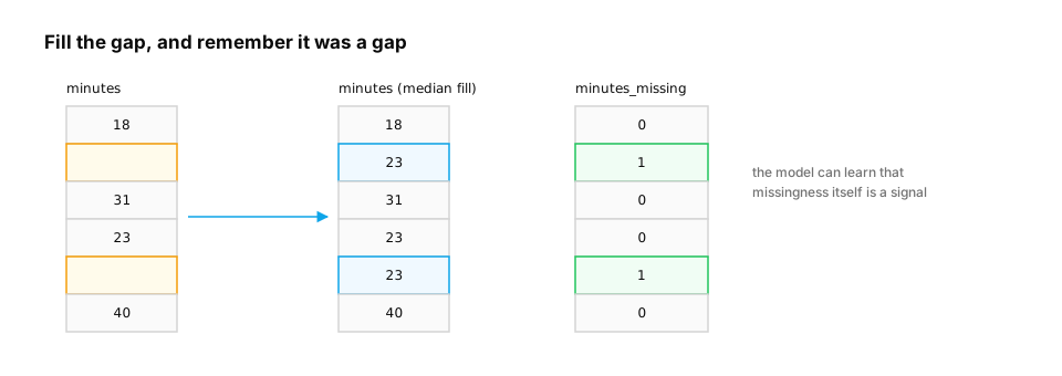
Worked example.
import numpy as np
from sklearn.impute import SimpleImputer

minutes = np.array([[12.0], [np.nan], [30.0], [8.0], [np.nan], [45.0]])
imputer = SimpleImputer(strategy="median", add_indicator=True)
print(imputer.fit_transform(minutes))
# column 0: missing values replaced by the median (21.0); column 1: 1.0 where the value was missing
Common trap. Filling missing values with 0 when 0 is a real, meaningful value ("zero minutes" ≠ "unknown").
2. Categorical features: encoding text labels as numbers
The question. How does a model use plan = "free" / "pro_monthly" / "pro_yearly" or country = "IN" / "US" / …?
Start from nothing.
- One-hot encoding — one 0/1 column per category. Safe and simple; explodes with many categories.
- Ordinal encoding — map categories to integers. Only correct when order is real (
beginner < intermediate < advanced); otherwise it invents a fake ordering for linear models (trees cope better). - Target encoding — replace each category with the average label for that category. Powerful for high-cardinality features (thousands of IDs), but it uses the label, so it must be computed out-of-fold or it leaks.
- Hashing / embeddings — for huge vocabularies (D4 learns embeddings end-to-end).
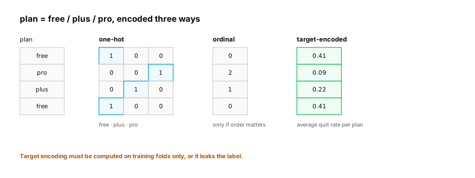
Worked example.
import pandas as pd
from sklearn.preprocessing import OneHotEncoder, OrdinalEncoder

df = pd.DataFrame({"plan": ["free", "pro_monthly", "free", "pro_yearly"],
                   "level": ["beginner", "advanced", "intermediate", "beginner"]})

onehot = OneHotEncoder(handle_unknown="ignore", sparse_output=False).fit(df[["plan"]])
print(onehot.get_feature_names_out(), onehot.transform(pd.DataFrame({"plan": ["pro_yearly", "enterprise"]})))
# an unseen category ("enterprise") becomes all zeros instead of crashing in production

ordinal = OrdinalEncoder(categories=[["beginner", "intermediate", "advanced"]])
print(ordinal.fit_transform(df[["level"]]).ravel())          # [0. 2. 1. 0.] — real order
3. Scaling: standardization and normalization
The question. One feature is "minutes" (5–60), another "tokens" (100–100,000). Does that matter?
Start from nothing.
- Standardization —
(x − mean) / std: mean 0, standard deviation 1. - Min–max normalization — rescale to [0, 1].
- Log transform — for heavy-tailed positive values (token counts, prices) before scaling.
Distance-based and gradient-based models (k-means, kNN, logistic regression, neural nets) are sensitive to scale; tree models are not (a split threshold works in any units). As with imputation, fit the scaler on training data only.
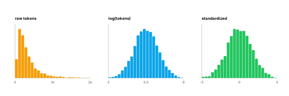
Worked example — scale changes k-nearest-neighbour results:
import numpy as np
from sklearn.model_selection import cross_val_score
from sklearn.neighbors import KNeighborsClassifier
from sklearn.pipeline import make_pipeline
from sklearn.preprocessing import StandardScaler

rng = np.random.default_rng(0)
n = 1000
minutes = rng.uniform(5, 60, n)
tokens = rng.uniform(100, 100_000, n)             # huge scale, but pure noise
y = minutes > 30                                  # the label depends only on minutes
X = np.column_stack([minutes, tokens])

print("kNN raw     :", cross_val_score(KNeighborsClassifier(), X, y, cv=5).mean().round(3))
print("kNN scaled  :", cross_val_score(make_pipeline(StandardScaler(), KNeighborsClassifier()), X, y, cv=5).mean().round(3))
Without scaling, distances are dominated by the noisy large-scale feature.
4. Building features: interactions, ratios and time
The question. The raw columns are there. What new columns would make the pattern obvious to the model?
Start from nothing. Good features encode domain knowledge:
- Ratios —
hints_per_lesson,tokens_per_second: often more meaningful than raw counts. - Interactions —
is_pro × lessons_done: "pro users who are active" behave differently. - Time features — hour of day, weekday, days since signup, days since last visit (recency), counts in the last 7 days (frequency). Cyclical values like hour of day can be encoded as
sin/cosso 23:00 is close to 00:00. - Aggregates — per-user averages and counts, computed only from events before the prediction time.
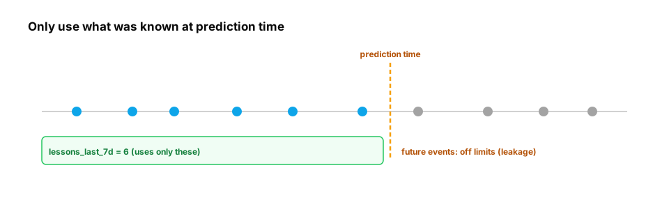
Worked example — recency/frequency features with a strict cut-off:
import pandas as pd

events = pd.DataFrame({
    "user": ["a", "a", "a", "b", "b", "c"],
    "ts": pd.to_datetime(["2026-10-01", "2026-10-20", "2026-11-05", "2026-10-02", "2026-10-03", "2026-11-06"]),
    "lesson_done": [1, 1, 0, 1, 1, 1],
})
prediction_time = pd.Timestamp("2026-11-01")
past = events[events.ts < prediction_time]                       # never look past the cut-off

features = past.groupby("user").agg(
    lessons_done=("lesson_done", "sum"),
    last_seen=("ts", "max"),
    active_days=("ts", "nunique"),
)
features["days_since_last_seen"] = (prediction_time - features.last_seen).dt.days
print(features.drop(columns="last_seen"))
# user "c" has no events before the cut-off, so has no row — handle as a cold-start user
5. Data leakage: when the model cheats
The question. A model scores 99% in testing and fails in production. What happened?
Start from nothing. Leakage is any information available during training that won't be available at prediction time. Common forms:
- Target leakage — a feature derived from the outcome (
cancellation_reasonto predict cancellation; "refund issued" to predict fraud). - Temporal leakage — features computed with future data, or a random split of time-ordered data.
- Preprocessing leakage — fitting the scaler, imputer, encoder or feature selection on the whole dataset before splitting.
- Duplicate/group leakage — the same user (or near-duplicate documents) in both train and test.
The fix: put every learned preprocessing step inside a Pipeline that is fit on training folds only, split by time or by group when appropriate, and ask of every feature: "Would I know this value at the moment I make the prediction?"
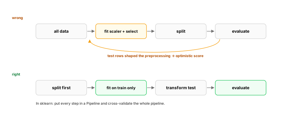
Worked example — feature selection leakage makes pure noise look predictive:
import numpy as np
from sklearn.feature_selection import SelectKBest, f_classif
from sklearn.linear_model import LogisticRegression
from sklearn.model_selection import cross_val_score
from sklearn.pipeline import make_pipeline

rng = np.random.default_rng(0)
X = rng.normal(size=(200, 5000))          # 5,000 random features
y = rng.integers(0, 2, 200)               # random labels: nothing to learn

# WRONG: choose the 20 "best" features using ALL rows, then cross-validate
X_leaky = SelectKBest(f_classif, k=20).fit_transform(X, y)
wrong = cross_val_score(LogisticRegression(max_iter=1000), X_leaky, y, cv=5).mean()

# RIGHT: selection happens inside each training fold
pipe = make_pipeline(SelectKBest(f_classif, k=20), LogisticRegression(max_iter=1000))
right = cross_val_score(pipe, X, y, cv=5).mean()

print(f"leaky accuracy {wrong:.2f}  vs  honest accuracy {right:.2f}   (truth: 0.50, it's noise)")
In production / interviews. Interview question: "Your churn model has 0.98 AUC offline but performs like chance in production. What do you check first?" (Leakage: feature timestamps relative to the label, preprocessing fit on all data, users appearing in both splits.)
6. Training-serving skew and feature stores
The question. The model is fine offline. In production, the same user gets a different prediction. Why?
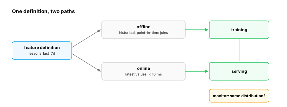
Start from nothing. Training-serving skew is when features are computed differently at training time (often a batch SQL job over history) and at serving time (often application code on live data). Typical causes: different code paths, different time windows, unit mismatches, a missing-value default that differs, or stale data.
Defences:
- One definition per feature, reused for training and serving — at minimum, save the fitted preprocessing pipeline with the model.
- Feature stores (Feast, Tecton, Vertex/SageMaker feature stores) keep feature definitions in one place, compute them for offline training with point-in-time correctness, and serve the latest values online with low latency (D11).
- Log the features actually served, and compare their distributions with the training data (monitoring, D11).
Worked example — save the fitted pipeline, not just the model:
import pickle
import numpy as np
import pandas as pd
from sklearn.compose import ColumnTransformer
from sklearn.impute import SimpleImputer
from sklearn.linear_model import LogisticRegression
from sklearn.pipeline import Pipeline, make_pipeline
from sklearn.preprocessing import OneHotEncoder, StandardScaler

rng = np.random.default_rng(1)
train = pd.DataFrame({"minutes": rng.uniform(5, 60, 500),
                      "plan": rng.choice(["free", "pro_monthly", "pro_yearly"], 500)})
train.loc[rng.random(500) < 0.1, "minutes"] = np.nan
y = (train.minutes.fillna(30) < 20) | (train.plan == "free")

preprocess = ColumnTransformer([
    ("num", make_pipeline(SimpleImputer(strategy="median"), StandardScaler()), ["minutes"]),
    ("cat", OneHotEncoder(handle_unknown="ignore"), ["plan"]),
])
model = Pipeline([("features", preprocess), ("clf", LogisticRegression())]).fit(train, y)

blob = pickle.dumps(model)                        # ship THIS: preprocessing + model together
served = pickle.loads(blob)
live_request = pd.DataFrame({"minutes": [np.nan], "plan": ["enterprise"]})   # missing + unseen
print("P(quit):", served.predict_proba(live_request)[0, 1].round(3))          # no crash, same logic as training
7. Feature selection and importance
The question. We have 300 candidate features. Should we keep them all?
Start from nothing. Fewer features → simpler, faster, less overfitting, easier monitoring. Approaches:
- Filter — score each feature alone (correlation, mutual information). Fast, ignores interactions.
- Embedded — L1 regularization zeroes weak features; tree models report importances.
- Permutation importance — shuffle one feature on held-out data and measure how much the score drops. Model-agnostic and honest — but correlated features share credit, so each can look unimportant alone.
Importance says what the model relies on, not what causes the outcome.
Worked example.
import numpy as np
from sklearn.ensemble import RandomForestClassifier
from sklearn.inspection import permutation_importance
from sklearn.model_selection import train_test_split

rng = np.random.default_rng(2)
n = 2000
useful = rng.normal(size=n)
copy_of_useful = useful + 0.05 * rng.normal(size=n)       # highly correlated duplicate
noise = rng.normal(size=(n, 3))
X = np.column_stack([useful, copy_of_useful, noise])
y = useful + 0.3 * rng.normal(size=n) > 0

X_tr, X_te, y_tr, y_te = train_test_split(X, y, random_state=0)
rf = RandomForestClassifier(n_estimators=200, random_state=0).fit(X_tr, y_tr)
perm = permutation_importance(rf, X_te, y_te, n_repeats=10, random_state=0)
for name, imp in zip(["useful", "copy_of_useful", "noise1", "noise2", "noise3"], perm.importances_mean):
    print(f"{name:15s} {imp:.3f}")
# the two correlated features split the credit; dropping one barely hurts the model
Quick check
A churn model's top feature is 'number of cancellation-page visits', and it predicts perfectly offline but poorly in production. What's likely happening?
Show the answer
B. Target leakage: the feature is recorded during the churn process itself (after or at the moment of the decision), so it isn't available early enough at prediction time — Features must be computable at prediction time from past data; leaked features inflate offline metrics and vanish in production.
Check yourself
- Recall: Why must an imputer or scaler be fitted on training data only?
- Apply: A feature
refund_issuedpredicts fraud with 99% accuracy. Use it? - Predict: Does standardizing features change a decision tree's accuracy?
Answers
- Otherwise statistics from validation/test data leak into training, inflating scores.
- Only if a refund is known before the fraud decision — usually it's a consequence of fraud, i.e. target leakage.
- No (essentially) — tree splits are thresholds and work the same in any monotonic rescaling.
Exercise
Build a churn pipeline on synthetic event data: compute recency/frequency features with a strict prediction-time cut-off, one-hot encode the plan, impute and scale numeric features inside a ColumnTransformer, and evaluate with a time-based split. Then deliberately add a leaky feature (days_until_cancel, computed using future events) and show how much it inflates the offline score.
Solution sketch
import numpy as np
import pandas as pd
from sklearn.compose import ColumnTransformer
from sklearn.ensemble import HistGradientBoostingClassifier
from sklearn.impute import SimpleImputer
from sklearn.metrics import roc_auc_score
from sklearn.pipeline import Pipeline
from sklearn.preprocessing import OneHotEncoder

rng = np.random.default_rng(0)
n = 4000
df = pd.DataFrame({
    "signup_month": rng.integers(1, 13, n),
    "plan": rng.choice(["free", "pro_monthly", "pro_yearly"], n, p=[0.7, 0.2, 0.1]),
    "days_since_last_seen": rng.exponential(7, n),
    "lessons_last_30d": rng.poisson(4, n).astype(float),
})
df.loc[rng.random(n) < 0.05, "lessons_last_30d"] = np.nan
logit = 0.15 * df.days_since_last_seen - 0.3 * df.lessons_last_30d.fillna(2) + (df.plan == "free") * 0.8 - 1
df["churned"] = rng.random(n) < 1 / (1 + np.exp(-logit))
df["days_until_cancel"] = np.where(df.churned, rng.integers(1, 30, n), 999)   # LEAKY: from the future

train, test = df[df.signup_month <= 9], df[df.signup_month > 9]               # time-based split

def evaluate(cols):
    num = [c for c in cols if c != "plan"]
    pre = ColumnTransformer([("num", SimpleImputer(strategy="median"), num),
                             ("cat", OneHotEncoder(handle_unknown="ignore"), ["plan"])])
    model = Pipeline([("pre", pre), ("gb", HistGradientBoostingClassifier(random_state=0))])
    model.fit(train[cols], train.churned)
    return roc_auc_score(test.churned, model.predict_proba(test[cols])[:, 1])

honest = ["plan", "days_since_last_seen", "lessons_last_30d"]
print(f"honest AUC {evaluate(honest):.3f} | with leaky feature {evaluate(honest + ['days_until_cancel']):.3f}")
This unlocks:
- ML evaluation — splitting and scoring so leaks are caught.
- D11 Feature engineering infrastructure — feature stores and point-in-time joins at scale.
- D16 Data processing & quality — data validation before features are built.
Sources: scikit-learn user guide — preprocessing, pipelines, "Common pitfalls and recommended practices" (data leakage), permutation importance; Kaufman et al., Leakage in Data Mining (2012); Sculley et al., Hidden Technical Debt in Machine Learning Systems (2015); Feast documentation — point-in-time joins.