
You already know: a layer is W x + b (D2 Linear algebra §3); backprop computes gradients through a graph (D2 Calculus §4); vanishing gradients and clipping (D2 Calculus §5); a 2-layer network solved XOR where a linear model couldn't (Bridge D3 → D4).
Why this matters for Atlas. Every LLM is a very deep neural network. Its building blocks — linear layers, activations, normalization, residual connections, careful initialization — are all on this page. Get these right and a 100-layer network trains smoothly; get one wrong and it silently fails to learn.
PyTorch examples run on CPU in a few seconds (
pip install torch).
1. From a perceptron to a multilayer network
The question. What is a "neuron", and why stack them?
Start from nothing. A single neuron computes a weighted sum and passes it through a nonlinear function: a = φ(w·x + b). A layer is many neurons side by side — exactly a matrix multiply plus a nonlinearity: h = φ(W x + b). A multilayer perceptron (MLP) stacks layers: ŷ = W₃ φ(W₂ φ(W₁ x + b₁) + b₂) + b₃.
Why the nonlinearity? Without it, stacked layers collapse into one matrix (W₃W₂W₁ is just another matrix) — no more powerful than linear regression. With it, each layer can bend and fold the space, and with enough hidden units an MLP can approximate any reasonable function (the universal approximation theorem). Depth lets it build features from features: edges → shapes → objects, or characters → words → meaning.
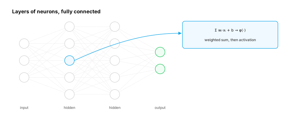
Real-life analogy. An assembly line of specialists: the first station sorts raw parts, the next assembles sub-components, the last builds the product. No single station does everything.
Worked example — the same MLP in NumPy (forward pass) and PyTorch (training):
import numpy as np
import torch
from torch import nn

torch.manual_seed(0)
rng = np.random.default_rng(0)

# Two interleaved spirals: hopeless for a linear model
n = 1000
t = rng.uniform(0, 3 * np.pi, n)
cls = rng.integers(0, 2, n)
X = np.column_stack([t * np.cos(t + np.pi * cls), t * np.sin(t + np.pi * cls)]) / 10
X += rng.normal(0, 0.02, X.shape)

model = nn.Sequential(nn.Linear(2, 64), nn.ReLU(), nn.Linear(64, 64), nn.ReLU(), nn.Linear(64, 2))
Xt, yt = torch.tensor(X, dtype=torch.float32), torch.tensor(cls)
opt = torch.optim.AdamW(model.parameters(), lr=1e-2)
for step in range(1500):
    loss = nn.functional.cross_entropy(model(Xt), yt)
    opt.zero_grad(); loss.backward(); opt.step()
acc = (model(Xt).argmax(1) == yt).float().mean().item()
print(f"MLP accuracy on spirals: {acc:.3f}  (final loss {loss.item():.3f})")

# The forward pass is just matrix multiplies + ReLU — redo it in NumPy with the learned weights
W = [layer.weight.detach().numpy() for layer in model if isinstance(layer, nn.Linear)]
b = [layer.bias.detach().numpy() for layer in model if isinstance(layer, nn.Linear)]
h = np.maximum(0, X @ W[0].T + b[0]); h = np.maximum(0, h @ W[1].T + b[1]); logits = h @ W[2].T + b[2]
print("NumPy forward pass agrees:", np.allclose(logits, model(Xt).detach().numpy(), atol=1e-5))
Common trap. "More parameters = better." A huge MLP memorizes small datasets; the evaluation discipline from D3 still decides.
2. Activation functions
The question. Which nonlinearity should go between layers?
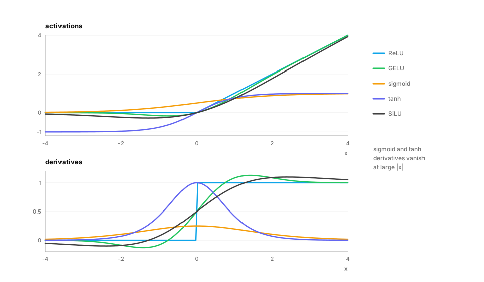
Start from nothing. The activation decides how signals and gradients flow:
| Activation | Formula | Gradient behaviour | Used in |
|---|---|---|---|
| Sigmoid | 1 / (1 + e^{−x}) |
≤ 0.25, vanishes for large |x| | Output layer for probabilities, gates |
| Tanh | (eˣ − e^{−x}) / (eˣ + e^{−x}) |
≤ 1, vanishes for large |x| | RNN/LSTM internals |
| ReLU | max(0, x) |
1 for x > 0, 0 otherwise ("dead" units possible) | CNNs, many MLPs |
| GELU | x · Φ(x) (Φ = normal CDF) |
smooth, slightly negative for small x < 0 | BERT, GPT-2/3, many transformers |
| SiLU / Swish | x · σ(x) |
smooth, like GELU | LLaMA-family (inside SwiGLU) |
ReLU fixed the vanishing-gradient problem of sigmoid/tanh in deep networks; GELU and SiLU are smooth versions that train slightly better in transformers.
Worked example — gradients through a stack of 20 layers:
import torch

torch.manual_seed(0)
for name, act in [("sigmoid", torch.sigmoid), ("tanh", torch.tanh),
                  ("relu", torch.relu), ("gelu", torch.nn.functional.gelu), ("silu", torch.nn.functional.silu)]:
    x = torch.randn(256, 128, requires_grad=True)
    h = x
    for _ in range(20):
        W = torch.randn(128, 128) * (2 / 128) ** 0.5          # He-style init (section 4)
        h = act(h @ W)
    h.sum().backward()
    print(f"{name:7s}: input-gradient size after 20 layers = {x.grad.abs().mean():.2e}")
Output: sigmoid ≈ 7e-11 (vanished), tanh ≈ 1.4, ReLU ≈ 1.8, GELU ≈ 0.7, SiLU ≈ 0.05. Sigmoid's gradient all but disappears through 20 layers; tanh, ReLU and GELU keep it alive at this initialization, and SiLU shrinks it somewhat. Whether gradients survive depends on the activation and the weight scale together — which is why initialization (section 4), normalization (section 5) and residual connections (section 6) are used together in real networks.
3. Loss functions and their numerics
The question. Which loss should a network minimize, and why do frameworks take raw scores (logits) instead of probabilities?
Start from nothing.
- Regression: mean squared error (MSE), or Huber loss (quadratic for small errors, linear for large — robust to outliers).
- Binary classification: binary cross-entropy. Use
BCEWithLogitsLoss— it fuses sigmoid + log in a numerically stable way. - Multi-class (and next-token prediction): cross-entropy on logits (
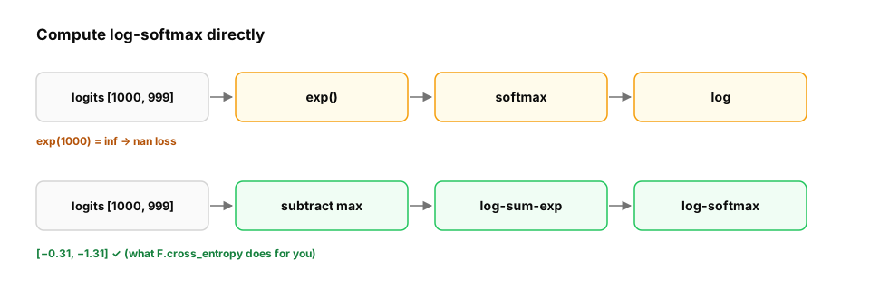
F.cross_entropy), which fuses softmax + log via the log-sum-exp trick. Computingsoftmaxand thenlogseparately can overflow (e^{1000}) or producelog(0) = −∞.
Worked example.
import torch
import torch.nn.functional as F

logits = torch.tensor([[1000.0, 0.0, -1000.0]])
target = torch.tensor([1])

naive = -torch.log(torch.softmax(logits, dim=1)[0, target])      # softmax underflows to 0 -> log(0)
stable = F.cross_entropy(logits, target)                          # uses log-sum-exp internally
print("naive :", naive.item())                                    # inf
print("stable:", stable.item())                                   # 1000.0

# log-sum-exp by hand: log(sum(e^z)) = m + log(sum(e^(z - m)))
m = logits.max()
lse = m + torch.log(torch.exp(logits - m).sum())
print("by hand:", (lse - logits[0, 1]).item())                    # 1000.0
4. Initialization: starting at the right scale
The question. If every weight starts at 0, or at a large random value, what goes wrong?
Start from nothing.
- All zeros: every neuron in a layer computes the same thing and gets the same gradient — they never become different (symmetry).
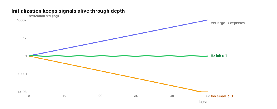
- Too large / too small random values: activations grow or shrink by a constant factor per layer, so after 50 layers they explode or vanish.
The fix is to choose the random scale so the variance of activations stays roughly constant across layers. With fan_in inputs per neuron:
- Xavier/Glorot:
Var(w) = 2 / (fan_in + fan_out)— for tanh/sigmoid. - He/Kaiming:
Var(w) = 2 / fan_in— for ReLU (which zeroes half its inputs, so it needs twice the variance).
Worked example.
import torch

torch.manual_seed(0)
x0 = torch.randn(512, 256)
for label, scale in [("std 0.01", lambda n: 0.01), ("std 0.1", lambda n: 0.1), ("He: sqrt(2/n)", lambda n: (2 / n) ** 0.5)]:
    h = x0
    stds = []
    for layer in range(30):
        W = torch.randn(256, 256) * scale(256)
        h = torch.relu(h @ W)
        stds.append(h.std().item())
    print(f"{label:14s} activation std at layers 1/10/30: {stds[0]:.2e} {stds[9]:.2e} {stds[29]:.2e}")
PyTorch's nn.Linear already uses a sensible default (Kaiming-uniform variant); transformers often use small normal init (std ≈ 0.02) plus scaled residual branches.
5. Normalization: BatchNorm, LayerNorm, RMSNorm
The question. Even with good initialization, activations drift during training. How do deep networks keep them in range?
Start from nothing. A normalization layer rescales activations to mean ≈ 0 and variance ≈ 1, then applies a learned scale (γ) and shift (β):
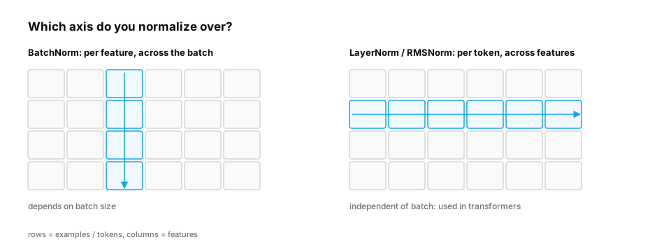
- BatchNorm — normalizes each feature across the batch. Great for CNNs; awkward for small batches and variable-length sequences, and behaves differently in training vs inference.
- LayerNorm — normalizes across the features of each token independently. The standard in transformers (works with any batch size).
- RMSNorm — LayerNorm without the mean subtraction:
x / √(mean(x²) + ε) · γ. Cheaper, works as well; used in LLaMA and most modern LLMs.
Worked example — implementing LayerNorm and RMSNorm and checking them:
import torch

torch.manual_seed(0)
x = torch.randn(4, 8) * 5 + 3                    # 4 tokens, 8 features, off-centre and wide

def layer_norm(x, gamma, beta, eps=1e-5):
    mean = x.mean(-1, keepdim=True)
    var = x.var(-1, keepdim=True, unbiased=False)
    return (x - mean) / torch.sqrt(var + eps) * gamma + beta

def rms_norm(x, gamma, eps=1e-6):
    return x / torch.sqrt((x ** 2).mean(-1, keepdim=True) + eps) * gamma

gamma, beta = torch.ones(8), torch.zeros(8)
ours = layer_norm(x, gamma, beta)
ref = torch.nn.LayerNorm(8, elementwise_affine=False)(x)
print("matches nn.LayerNorm:", torch.allclose(ours, ref, atol=1e-5))
print("per-token mean ≈ 0:", ours.mean(-1).abs().max().item() < 1e-5, "| std ≈ 1:", ours.std(-1, unbiased=False).round(decimals=3).tolist())
print("RMSNorm per-token RMS:", torch.sqrt((rms_norm(x, gamma) ** 2).mean(-1)).round(decimals=3).tolist())
6. Regularization and residual connections
The question. How do we stop a big network from memorizing — and how do 100-layer networks train at all?
Start from nothing.
- Dropout — during training, randomly zero a fraction
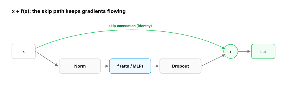
pof activations (and scale the rest by1/(1−p)), so the network can't rely on any single unit; at inference, dropout is off. Also: weight decay (AdamW), data augmentation, early stopping. - Residual connections — instead of
h = f(x), computeh = x + f(x). The layer only has to learn a change to its input, and gradients get a direct "highway" backwards (the derivative ofx + f(x)with respect toxincludes a1). This is what made very deep networks (ResNet, 2015) and every transformer trainable.
Transformers combine them as: x = x + Dropout(Attention(Norm(x))), then x = x + Dropout(MLP(Norm(x))) — the "pre-norm residual block".
Worked example — gradient flow with and without residuals, and dropout's train/eval difference:
import torch
from torch import nn

torch.manual_seed(0)

def first_layer_grad(residual, depth=50, width=64):
    layers = [nn.Sequential(nn.Linear(width, width), nn.Tanh()) for _ in range(depth)]
    x = torch.randn(32, width)
    h = x
    for f in layers:
        h = h + f(h) if residual else f(h)
    h.pow(2).mean().backward()
    return layers[0][0].weight.grad.abs().mean().item()

print(f"50 plain layers    : first-layer gradient {first_layer_grad(False):.2e}")
print(f"50 residual layers : first-layer gradient {first_layer_grad(True):.2e}")

drop = nn.Dropout(p=0.5)
x = torch.ones(1, 10)
drop.train(); print("train mode:", drop(x))      # about half zeroed, survivors scaled to 2.0
drop.eval();  print("eval mode :", drop(x))      # unchanged
Common trap. Forgetting model.eval() at inference: dropout keeps dropping and BatchNorm uses batch statistics, so predictions become random and batch-dependent.
In production / interviews. Interview question: "Why do transformers use pre-norm residual blocks with LayerNorm/RMSNorm rather than BatchNorm?" (Batch-size independence, variable-length sequences, stable gradients through residual highways in very deep stacks.)
Quick check
A deep ReLU network initialized with weights from N(0, 1) produces activations that explode layer by layer. What's the fix?
Show the answer
D. Scale initial weights by sqrt(2 / fan_in) (He initialization) so activation variance stays roughly constant across layers — Each layer multiplies variance by fan_in × Var(w)/2 for ReLU; He initialization makes that factor about 1.
Check yourself
- Recall: Why must there be a nonlinearity between linear layers?
- Apply: You're stacking 40 ReLU layers. Which initialization?
- Predict: What does
F.cross_entropyreturn for logits[0, 0, 0, 0]and any target?
Answers
- Without it, the composition of linear layers is a single linear map — no extra expressive power.
- He/Kaiming (variance 2/fan_in), ideally with residual connections and normalization.
ln 4 ≈ 1.386— a uniform distribution over 4 classes gives each probability ¼.
Exercise
Build a 12-layer MLP classifier in PyTorch for the spiral data with a configurable block: Linear → (optional) LayerNorm → activation → (optional) Dropout, with an optional residual connection. Train four variants (plain, +residual, +residual+LayerNorm, +all with dropout 0.1) for the same number of steps and compare final training loss and validation accuracy.
Solution sketch
import numpy as np
import torch
from torch import nn

torch.manual_seed(0); rng = np.random.default_rng(0)
n = 2000
t = rng.uniform(0, 3 * np.pi, n); c = rng.integers(0, 2, n)
X = np.column_stack([t * np.cos(t + np.pi * c), t * np.sin(t + np.pi * c)]) / 10 + rng.normal(0, 0.03, (n, 2))
X, y = torch.tensor(X, dtype=torch.float32), torch.tensor(c)
tr, va = slice(0, 1600), slice(1600, None)

class Block(nn.Module):
    def __init__(self, w, norm, drop, residual):
        super().__init__()
        self.lin, self.norm = nn.Linear(w, w), nn.LayerNorm(w) if norm else nn.Identity()
        self.drop, self.residual = nn.Dropout(drop), residual
    def forward(self, x):
        out = self.drop(nn.functional.gelu(self.norm(self.lin(x))))
        return x + out if self.residual else out

def make(norm=False, drop=0.0, residual=False, depth=12, w=64):
    return nn.Sequential(nn.Linear(2, w), *[Block(w, norm, drop, residual) for _ in range(depth)], nn.Linear(w, 2))

for name, cfg in {"plain": {}, "+residual": dict(residual=True), "+res+norm": dict(residual=True, norm=True),
                  "+res+norm+dropout": dict(residual=True, norm=True, drop=0.1)}.items():
    torch.manual_seed(0); m = make(**cfg); opt = torch.optim.AdamW(m.parameters(), lr=3e-3)
    for _ in range(600):
        m.train(); loss = nn.functional.cross_entropy(m(X[tr]), y[tr]); opt.zero_grad(); loss.backward(); opt.step()
    m.eval(); acc = (m(X[va]).argmax(1) == y[va]).float().mean().item()
    print(f"{name:18s} train loss {loss.item():.3f}  val acc {acc:.3f}")
At 12 layers with AdamW, all four variants reach ≈97% — adaptive optimizers and GELU are forgiving at this depth. Set depth=50 and the plain network stalls at loss 0.693 (= ln 2, a coin flip) and ~49% accuracy, while every residual variant still reaches ~97%: the benefit of these components grows with depth.
This unlocks:
- Major architectures — CNNs, RNNs and transformers built from these blocks.
- PyTorch engineering — what
nn.Module, autograd and mixed precision do under the hood. - D5 Transformer architecture — pre-norm residual blocks with RMSNorm and SwiGLU.
Sources: Goodfellow et al., Deep Learning (ch. 6–8); Glorot & Bengio (2010) and He et al. (2015) on initialization; Ioffe & Szegedy, Batch Normalization (2015); Ba et al., Layer Normalization (2016); Zhang & Sennrich, RMSNorm (2019); Srivastava et al., Dropout (2014); He et al., Deep Residual Learning (2015); Hendrycks & Gimpel, GELU (2016).