VFlash: Fast, Accurate Visual Planning via Flash Primitive Decoding
u_Unrolled
D4: Deep Learning · Autograd From Scratch, and Debugging Training — Gradient Checks, Loss Curves and the Usual Bugs
Phase 3/Domain 4/Lesson 2

Autograd From Scratch, and Debugging Training — Gradient Checks, Loss Curves and the Usual Bugs

15 min read·Intermediate· Unrolled Pro
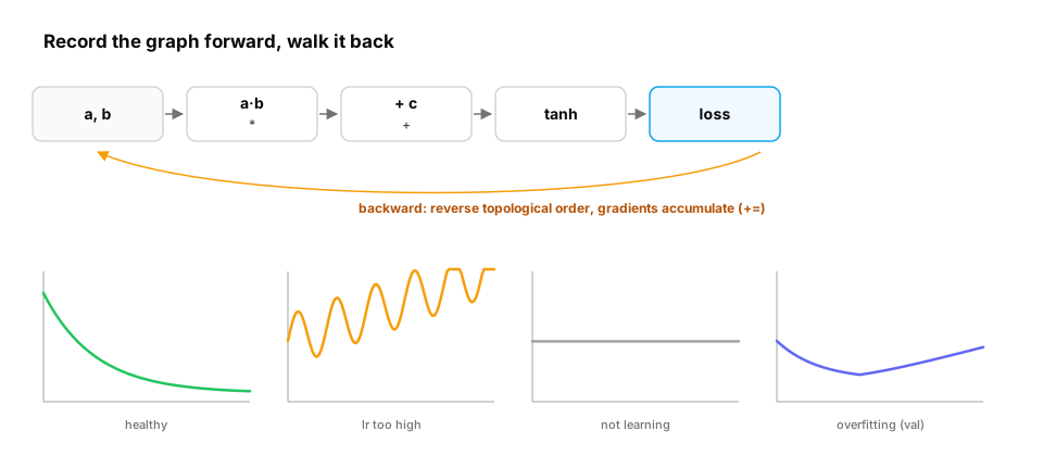
a computation graph for a tiny network built during the forward pass (nodes for multiply, add, tanh, loss), then traversed in reverse topological order, each node passing its local gradient back to its inputs; beside it, four loss curves annotated with their diagnoses: healthy, learning rate too high, not learning (bug), and overfitting.
Diagram— a computation graph for a tiny network built during the forward pass (nodes for multiply, add, tanh, loss), then traversed in reverse topological order, each node passing its local gradient back to its inputs; beside it, four loss curves annotated with their diagnoses: healthy, learning rate too high, not learning (bug), and overfitting.

You already know: the chain rule and backpropagation (Calculus); Jacobians and vector–Jacobian products (Jacobians and Taylor); layers, activations, losses and initialization (Neural network fundamentals).

Why this matters for Atlas. PyTorch's autograd feels like magic until something goes wrong. Building a small version yourself (about 60 lines) shows exactly what happens: the forward pass records a graph, and the backward pass walks it in reverse, accumulating gradients. That understanding makes the debugging habits obvious: check gradients numerically, overfit a single batch, read loss curves, and know the dozen bugs that cause most failed runs. This lesson builds the engine, trains a network with it, and then walks through the debugging checklist, ending with the "write a training loop and attention from memory" exercise interviewers love.


1. A tiny autograd engine

The question. How does loss.backward() know what to do?

Start from nothing. Every operation creates a node that remembers its inputs and how to compute its local gradient. During backward(), we order the graph so each node comes after everything that depends on it (reverse topological order), seed the output's gradient with 1, and let each node push gradient to its inputs using the chain rule. Gradients accumulate (+=), because a value used in several places receives gradient from each use; that's also why real frameworks need you to zero gradients between steps.

That's the preview. The full lesson, with its code and exercises, is part of Unrolled Pro.
Staff AI & Pro Tier Lesson

Unlock "Autograd From Scratch, and Debugging Training — Gradient Checks, Loss Curves and the Usual Bugs"

The foundations are free forever. Unrolled Pro unlocks the complete lesson, production architectures, and 55 battle-tested ML system design case studies.

Everything included with Pro:
All 234+ Deep-Dive Lessons across transformer internals, inference, RAG & agents
55 Staff-Level ML & System Design Case Studies with mathematical capacity estimates
AI Engineer Sheet & Exercises with worked solutions, self-checks, and code
100 Landmark Research Papers guided walkthroughs & progress tracking
14-Day Money-Back Guarantee — 100% full refund if you aren't satisfied
View Plans & Unlock All Lessons

From ₹167/mo (~$2/mo) · Cancel anytime · Instant activation

100% Risk-Free: 14-day no-questions-asked money-back guarantee