You already know: convolutions and vision transformers (Computer vision); encoder–decoder transformers and next-token generation (D5); latency budgets, TTFT and streaming (D12, D1 Networking); evaluation per slice (D10).
Why this matters for Atlas. Voice is the most natural interface and the hardest to get right in real time. The pipeline turns a pressure wave into numbers (sampling), into a time–frequency picture (the spectrogram), into text (automatic speech recognition, ASR), and back from text into sound (text-to-speech, TTS), or skips text entirely in speech-to-speech models. Quality is measured differently (word error rate, naturalness), and latency is unforgiving: people expect a reply within a few hundred milliseconds of finishing a sentence. This lesson builds the signal processing from first principles, explains ASR and TTS architectures, computes WER, and designs a voice-agent latency budget.
1. Sound as numbers: sampling and frequency
The question. How does a microphone signal become something a model can process?
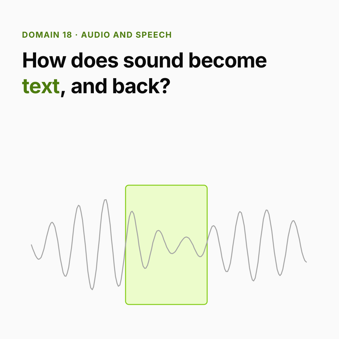
Start from nothing. Sound is air pressure varying over time. A microphone measures it thousands of times per second: the sample rate. By the Nyquist theorem, sampling at rate f captures frequencies up to f/2; speech information lies mostly below 8 kHz, so speech models usually use 16 kHz audio (music uses 44.1 or 48 kHz). Each sample is a number (16-bit integers or floats). One second of 16 kHz audio is 16,000 numbers: too long and too low-level to feed a model directly.