You already know: MDPs, returns, value functions and the Bellman equation (RL I); neural networks and gradient descent (D4).
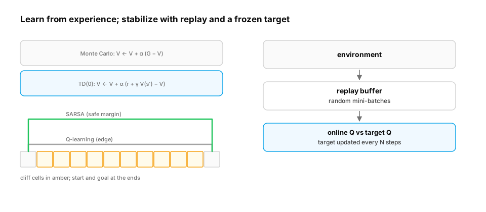
Why this matters for Atlas. Value iteration needs the model of the world. Model-free RL learns values from experience instead: Monte Carlo methods average complete returns; temporal-difference (TD) methods update from one step plus their own estimate of the rest (bootstrapping), learning faster and online. Q-learning learns the optimal action values even while behaving exploratorily, and DQN scales it to large state spaces with a neural network, made stable by a replay buffer and a target network. These ideas (bootstrapped value estimates, off-policy learning, stabilization tricks) reappear in the critics and advantage estimates of PPO for LLMs.
1. Monte Carlo vs temporal-difference learning
The question. How do you estimate a policy's value from episodes, without knowing P?
Start from nothing. Monte Carlo: run episodes, compute each visited state's actual return G, and move V(s) towards it: V(s) ← V(s) + α (G − V(s)). Unbiased, but high variance (a return sums many random rewards) and it must wait until the episode ends. TD(0): after each step, move V(s) towards the TD target r + γ V(s′): V(s) ← V(s) + α (r + γ V(s′) − V(s)). The bracket is the TD error δ. TD is biased (it trusts its own current estimate of V(s′)) but much lower variance, and it learns online. On the classic random walk, TD typically reaches lower error with the same number of episodes.
import numpy as np

n_states = 7                                                   # states 1..5 are non-terminal; 0 and 6 terminal
true_v = np.arange(1, 6) / 6                                   # P(ending on the right) from each state

def episode(rng):
    s, traj = 3, []
    while 0 < s < 6:
        s2 = s + (1 if rng.random() < 0.5 else -1)
        traj.append((s, 1.0 if s2 == 6 else 0.0, s2)); s = s2
    return traj

def run(method, alpha, episodes=100, seed=0):
    rng = np.random.default_rng(seed); V = np.full(n_states, 0.5); V[0] = V[6] = 0.0
    errors = []
    for _ in range(episodes):
        traj = episode(rng)
        if method == "MC":
            G = traj[-1][1]                                         # undiscounted; only the final step is rewarded
            for s, r, s2 in traj:
                V[s] += alpha * (G - V[s])
        else:
            for s, r, s2 in traj:
                V[s] += alpha * (r + V[s2] - V[s])
        errors.append(np.sqrt(np.mean((V[1:6] - true_v) ** 2)))
    return np.mean(errors[-20:])

for method, alpha in [("MC", 0.02), ("MC", 0.05), ("TD", 0.05), ("TD", 0.1)]:
    err = np.mean([run(method, alpha, seed=s) for s in range(100)])
    print(f"{method} alpha {alpha}: RMS error after 100 episodes {err:.3f}")
With comparable learning rates, TD's estimates are closer to the true values after the same number of episodes: bootstrapping trades a little bias for a large reduction in variance.
2. SARSA and Q-learning: learning to act
The question. How do you learn which actions to take, not just how good states are?
Start from nothing. Learn action values Q(s, a) and act ε-greedily. SARSA (on-policy) updates towards r + γ Q(s′, a′), where a′ is the action the agent will actually take next, so it learns the value of its exploratory behaviour. Q-learning (off-policy) updates towards r + γ maxₐ′ Q(s′, a′), the value of acting greedily afterwards, so it learns the optimal policy regardless of how it explores. The classic cliff-walking example shows the difference: Q-learning learns the shortest path along the cliff edge (optimal if you never explore), while SARSA learns a safer path that accounts for its own random steps, and earns more reward during training.
import numpy as np

H, W = 4, 12
start, goal = (3, 0), (3, 11)
moves = [(-1, 0), (1, 0), (0, -1), (0, 1)]

def step(s, a):
    r, c = s[0] + moves[a][0], s[1] + moves[a][1]
    r, c = min(max(r, 0), H - 1), min(max(c, 0), W - 1)
    if r == 3 and 0 < c < 11:
        return start, -100.0, False                             # fell off the cliff
    return (r, c), -1.0, (r, c) == goal

def train(method, episodes=500, alpha=0.5, eps=0.1, seed=0):
    rng = np.random.default_rng(seed); Q = np.zeros((H, W, 4)); returns = []
    pick = lambda s: rng.integers(4) if rng.random() < eps else int(np.argmax(Q[s]))
    for _ in range(episodes):
        s, a, total, done = start, pick(start), 0.0, False
        while not done:
            s2, r, done = step(s, a); total += r
            a2 = pick(s2)
            target = r if done else r + (Q[s2][a2] if method == "SARSA" else Q[s2].max())
            Q[s][a] += alpha * (target - Q[s][a])
            s, a = s2, a2
        returns.append(total)
    return Q, np.mean(returns[-100:])

def greedy_path_row(Q):
    s, rows = start, []
    for _ in range(40):
        s, _, done = step(s, int(np.argmax(Q[s]))); rows.append(s[0])
        if done:
            break
    return min(rows)

for method in ["SARSA", "Q-learning"]:
    res = [train(method, seed=sd) for sd in range(10)]
    rows = [greedy_path_row(Q) for Q, _ in res]
    print(f"{method:<11} average return per episode while exploring: {np.mean([r for _, r in res]):7.1f}; "
          f"highest row of the greedy path in 10 runs: {rows}")
print("(row 2 runs along the cliff edge; rows 1 and 0 keep a safety margin)")
Q-learning's greedy path hugs the cliff (the optimal route, 13 steps) but its ε-greedy behaviour keeps falling off during training, so its returns while learning are worse; SARSA learns a path farther from the edge in 9 of 10 runs (most of them along the top row), because its value estimates include its own exploration, and it loses half as much reward while learning.
Quick check
What is the key difference between the SARSA and Q-learning update targets?
Show the answer
A. SARSA bootstraps from Q(s′, a′) for the action actually taken next (on-policy); Q-learning bootstraps from max over a′ of Q(s′, a′), the greedy action (off-policy), so it learns the optimal policy regardless of exploration — The max in Q-learning's target makes it estimate the value of the greedy policy even while behaving ε-greedily; SARSA estimates the value of the policy it's actually following.
3. DQN: Q-learning with a neural network
The question. What breaks when Q is a neural network, and how did DQN fix it?
Start from nothing. Large state spaces (images, continuous sensors) need a function approximator Q_θ(s, a). Naively training it on consecutive transitions with the TD target is unstable: consecutive samples are highly correlated, and the target r + γ max Q_θ(s′, ·) moves every time θ changes, so the network chases its own tail. DQN (Mnih et al., 2015) added two fixes: an experience replay buffer (store transitions, train on random mini-batches, breaking correlations and reusing data) and a target network (compute targets with a frozen copy θ⁻ updated every N steps). Later improvements: Double DQN (decouple action selection from evaluation to reduce overestimation), prioritized replay, dueling networks.
import numpy as np

H, W = 5, 5
goal, trap = (0, 4), (2, 2)
moves = [(-1, 0), (1, 0), (0, -1), (0, 1)]

def env_step(s, a):
    r, c = min(max(s[0] + moves[a][0], 0), H - 1), min(max(s[1] + moves[a][1], 0), W - 1)
    if (r, c) == goal: return (r, c), 1.0, True
    if (r, c) == trap: return (r, c), -1.0, True
    return (r, c), -0.02, False

def feats(s):
    x = np.zeros(H * W); x[s[0] * W + s[1]] = 1.0; return x

def dqn(replay, target_net, episodes=100, seed=0, gamma=0.95, lr=0.2):
    rng = np.random.default_rng(seed)
    W1 = rng.standard_normal((H * W, 32)) * 0.3; W2 = rng.standard_normal((32, 4)) * 0.3
    tW1, tW2 = W1.copy(), W2.copy(); buf, steps = [], 0
    def q(x, A, B): h = np.maximum(x @ A, 0); return h, h @ B
    for ep in range(episodes):
        s, done, t = (4, 0), False, 0
        eps = max(0.05, 1 - ep / 200)
        while not done and t < 50:
            a = rng.integers(4) if rng.random() < eps else int(np.argmax(q(feats(s), W1, W2)[1]))
            s2, r, done = env_step(s, a); buf.append((feats(s), a, r, feats(s2), done)); s = s2; t += 1; steps += 1
            batch = [buf[i] for i in rng.integers(0, len(buf), 32)] if replay else [buf[-1]]
            X = np.array([b[0] for b in batch]); A = np.array([b[1] for b in batch]); R = np.array([b[2] for b in batch])
            X2 = np.array([b[3] for b in batch]); D = np.array([b[4] for b in batch], float)
            nxt = q(X2, tW1, tW2)[1] if target_net else q(X2, W1, W2)[1]
            y = R + gamma * (1 - D) * nxt.max(1)
            h, Q = q(X, W1, W2)
            g = np.zeros_like(Q); g[np.arange(len(A)), A] = (Q[np.arange(len(A)), A] - y) / len(A)
            dh = g @ W2.T * (h > 0)
            W2 -= lr * h.T @ g; W1 -= lr * X.T @ dh
            if target_net and steps % 100 == 0:
                tW1, tW2 = W1.copy(), W2.copy()
    # evaluate the greedy policy from the start
    s, total = (4, 0), 0.0
    for _ in range(30):
        s, r, done = env_step(s, int(np.argmax(q(feats(s), W1, W2)[1]))); total += r
        if done: break
    return total, s == goal

for replay, target in [(False, False), (True, False), (True, True)]:
    res = [dqn(replay, target, seed=sd) for sd in range(8)]
    print(f"replay={str(replay):<5} target net={str(target):<5}: greedy policy reaches the goal in {np.mean([g for _, g in res]):.0%} of runs, "
          f"mean return {np.mean([t for t, _ in res]):+.2f}")
With a short training budget, online updates on single, correlated transitions fail in a quarter of the runs; the replay buffer, which reuses each transition many times in decorrelated mini-batches, makes learning more reliable. The target network makes no difference here: with one-hot inputs, an update for one state barely changes the network's estimates for the others, so the targets hardly move. Its value appears at scale, when a network generalizes across millions of similar states (pixels, embeddings) and every update shifts the targets it is chasing, which is the regime where the original DQN needed it to avoid divergence.
Check yourself
- Write the Monte Carlo and TD(0) updates, and compare their bias and variance.
- What is the TD error?
- How do SARSA and Q-learning differ, and what does cliff walking show?
- Why is naive Q-learning with a neural network unstable?
- What do the replay buffer and target network each fix?
Answers
- MC: V ← V + α(G − V) using the full return (unbiased, high variance, waits for episode end). TD(0): V ← V + α(r + γV(s′) − V) (biased by bootstrapping, lower variance, online).
- δ = r + γV(s′) − V(s): the difference between the one-step bootstrapped target and the current estimate.
- SARSA bootstraps from the next action actually taken (on-policy); Q-learning from the greedy maximum (off-policy). Q-learning learns the risky optimal path and falls more during exploration; SARSA learns a safer path that accounts for exploration.
- Consecutive samples are correlated, and the target depends on the same parameters being updated, so the network chases a moving target and can diverge.
- Replay breaks correlations and reuses data; the target network holds the bootstrapped targets fixed between periodic updates.
Exercise
Add Double Q-learning to the cliff-walking agent: keep two tables Q_A and Q_B, act ε-greedily on their sum, and on each step update one of them at random using the other to evaluate its argmax action. Construct a small MDP where max-based targets overestimate (a state with ten actions whose rewards are all N(−0.1, 1) noise, so the true best value is −0.1), and show that Q-learning's estimate of that state is biased upwards while Double Q-learning's isn't.
Solution
import numpy as np

def estimate(double, steps=20_000, n_actions=10, alpha=0.1, seed=0):
    rng = np.random.default_rng(seed)
    QA, QB = np.zeros(n_actions), np.zeros(n_actions)              # Q-values of the noisy state B
    VA_start, VB_start = 0.0, 0.0                                  # value of the start state that leads to B
    for _ in range(steps):
        a = rng.integers(n_actions)                                # explore uniformly in B
        r = rng.normal(-0.1, 1.0)
        if not double:
            QA[a] += alpha * (r - QA[a])
            VA_start += alpha * (0 + QA.max() - VA_start)          # target uses max over noisy estimates
        else:
            if rng.random() < 0.5:
                QA[a] += alpha * (r - QA[a])
                VA_start += alpha * (QB[np.argmax(QA)] - VA_start)  # select with A, evaluate with B
            else:
                QB[a] += alpha * (r - QB[a])
                VA_start += alpha * (QA[np.argmax(QB)] - VA_start)
    return VA_start

ql = np.mean([estimate(False, seed=s) for s in range(20)])
dq = np.mean([estimate(True, seed=s) for s in range(20)])
print(f"true value of reaching the noisy state: -0.10; Q-learning estimate {ql:+.2f}; Double Q-learning estimate {dq:+.2f}")
Taking the maximum of ten noisy estimates picks whichever happens to be high, so Q-learning believes the noisy state is worth well above its true −0.1 and would be lured towards it. Double Q-learning selects the action with one estimate and evaluates it with an independent one, which removes that selection bias. The same idea is used in Double DQN and in the clipped double-Q critics of modern continuous-control methods.
This unlocks:
- RL III: policy gradients, actor-critic and PPO — learning policies directly, with value functions as critics.
Sources: Sutton & Barto, Reinforcement Learning: An Introduction (2nd ed.), ch. 5–6; Sutton, Learning to Predict by the Methods of Temporal Differences (1988); Watkins & Dayan, Q-learning (1992); Mnih et al., Human-level control through deep reinforcement learning (Nature 2015); van Hasselt, Double Q-learning (NeurIPS 2010) and van Hasselt, Guez & Silver, Deep RL with Double Q-learning (AAAI 2016).