You already know: probability, expectation and Bayes' rule (Probability); the Gaussian and the CLT (Joint distributions); A/B testing (D2, D10).
Why this matters for Atlas. Supervised learning is told the right answer; reinforcement learning only gets rewards for what it tried, so it must explore to discover good actions and exploit what it knows, and in multi-step problems it must assign credit for a reward to the decisions that led to it. Bandits isolate the exploration problem; Markov decision processes add sequential consequences. The Bellman equation, introduced here, is the idea behind every RL algorithm in this track, including the PPO and GRPO that post-train LLMs (D6).
1. Multi-armed bandits: explore or exploit?
The question. Five practice formats, unknown success rates. How do you learn the best while wasting as few students as possible on bad ones?
Start from nothing. Each arm gives a random reward with unknown mean. Regret is the reward lost compared with always playing the best arm. Pure exploitation gets stuck on an arm that looked good early; pure exploration (uniform A/B testing) wastes traffic on arms already known to be bad. Classic strategies:
- ε-greedy: exploit the best estimate, but with probability ε try a random arm.
- UCB (upper confidence bound): pick the arm with the highest optimistic estimate, mean + c·√(ln t / nₐ), so rarely tried arms get a bonus that shrinks as evidence accumulates.
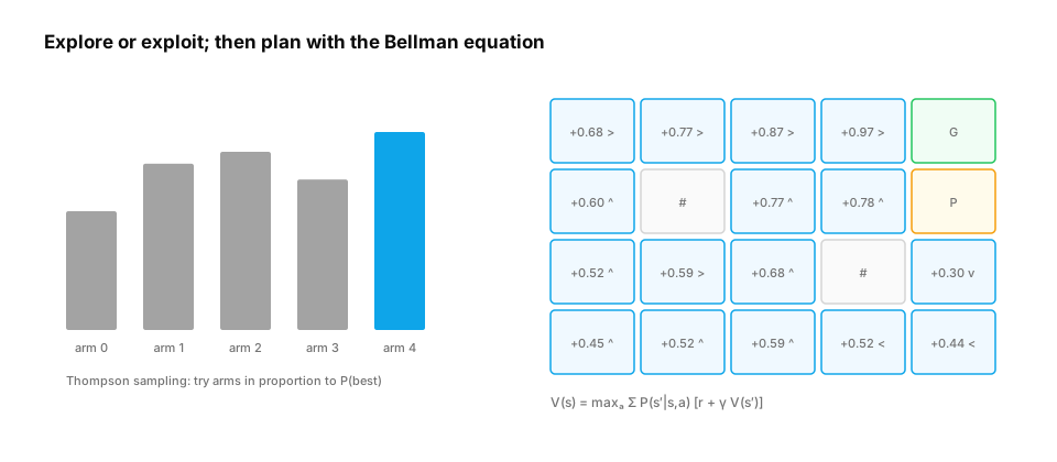
- Thompson sampling: keep a posterior over each arm's mean (Beta for success/failure), sample one value from each, play the best sample. It explores exactly as much as the uncertainty warrants and works very well in practice.
import numpy as np

true_p = np.array([0.30, 0.42, 0.45, 0.38, 0.50])         # success rate of each practice format
T, runs = 5000, 60

def run(policy, seed):
    rng = np.random.default_rng(seed)
    n, s = np.zeros(5), np.zeros(5); regret = 0.0
    for t in range(1, T + 1):
        if policy == "epsilon":
            a = rng.integers(5) if rng.random() < 0.1 or n.min() == 0 else np.argmax(s / n)
        elif policy == "ucb":
            a = int(np.argmin(n)) if n.min() == 0 else np.argmax(s / n + np.sqrt(2 * np.log(t) / n))
        else:                                                  # Thompson sampling with Beta(1 + successes, 1 + failures)
            a = np.argmax(rng.beta(1 + s, 1 + n - s))
        r = rng.random() < true_p[a]
        n[a] += 1; s[a] += r; regret += true_p.max() - true_p[a]
    return regret, n[4] / T

for policy in ["epsilon", "ucb", "thompson"]:
    res = np.array([run(policy, seed) for seed in range(runs)])
    print(f"{policy:<9} mean regret {res[:, 0].mean():6.1f} successes lost over {T} students; best arm chosen {res[:, 1].mean():.0%} of the time")
print(f"uniform A/B split would lose {T * (true_p.max() - true_p.mean()):.0f}")
All three beat a uniform split by a wide margin (UCB's bonus is conservative here and explores the close runners-up for longer); Thompson sampling loses the least, because its exploration shrinks automatically as the posteriors sharpen, while ε-greedy keeps exploring at a fixed 10% forever. Bandits are the right tool when you care about outcomes during the experiment (recommendation slots, prompt variants); a fixed A/B test is right when you need a clean, unbiased estimate of the difference.
2. Markov decision processes and returns
The question. What changes when actions affect the future?
Start from nothing. An MDP has states S, actions A, transition probabilities P(s′ | s, a), rewards R(s, a, s′) and a discount factor γ ∈ [0, 1). The Markov property: the next state depends only on the current state and action. A policy π(a | s) chooses actions. The return G_t = r_{t+1} + γ r_{t+2} + γ² r_{t+3} + … is the discounted sum of future rewards; γ trades off immediate against delayed reward (and keeps infinite sums finite). The value V^π(s) is the expected return from s under π; the action value Q^π(s, a) is the expected return after taking a in s and then following π. An LLM generating text is an MDP: the state is the prompt plus tokens so far, actions are tokens, and the reward (often) comes at the end (D6 RL for LLMs).
3. The Bellman equation, value iteration and policy iteration
The question. How do you compute the best policy when you know the MDP?
Start from nothing. Values satisfy a recursive consistency condition, the Bellman equation: V^π(s) = Σₐ π(a|s) Σ_{s′} P(s′|s,a) [R + γ V^π(s′)]. The optimal value satisfies V*(s) = maxₐ Σ_{s′} P(s′|s,a) [R + γ V*(s′)]. Value iteration applies this as an update until values stop changing (it's a contraction, so it converges), then acts greedily. Policy iteration alternates evaluating the current policy exactly and improving it greedily; it converges in few iterations. Both need the model P and R, which RL usually doesn't have: the next lesson learns from samples instead.
import numpy as np

H, W = 4, 5
walls, goal, pit = {(1, 1), (2, 3)}, (0, 4), (1, 4)
actions = [(-1, 0), (1, 0), (0, -1), (0, 1)]                      # up, down, left, right
arrows = "^v<>"
states = [(r, c) for r in range(H) for c in range(W) if (r, c) not in walls]
gamma, slip = 0.95, 0.1                                         # 10% of the time the move goes sideways

def step_probs(s, a):
    if s in (goal, pit):
        return [(s, 1.0)]
    outs = []
    for k, p in [(a, 1 - slip), ((a + 2) % 4, slip / 2), ((a + 3) % 4, slip / 2)]:
        dr, dc = actions[k]; nxt = (s[0] + dr, s[1] + dc)
        outs.append((nxt if nxt in states else s, p))
    return outs

def reward(s2, s):
    if s in (goal, pit):
        return 0.0
    return 1.0 if s2 == goal else (-1.0 if s2 == pit else -0.04)  # small cost per step

V = {s: 0.0 for s in states}
for it in range(500):
    delta = 0.0
    for s in states:
        best = max(sum(p * (reward(s2, s) + gamma * V[s2]) for s2, p in step_probs(s, a)) for a in range(4))
        delta = max(delta, abs(best - V[s])); V[s] = best
    if delta < 1e-8:
        break
policy = {s: max(range(4), key=lambda a: sum(p * (reward(s2, s) + gamma * V[s2]) for s2, p in step_probs(s, a))) for s in states}
print(f"value iteration converged in {it + 1} sweeps")
for r in range(H):
    print("  ".join(("  #  " if (r, c) in walls else " GOAL" if (r, c) == goal else " PIT " if (r, c) == pit
                     else f"{V[(r, c)]:+.2f}{arrows[policy[(r, c)]]}") for c in range(W)))
The values fall off with distance from the goal (discounting and step costs), and the greedy policy routes around the walls; next to the pit, it chooses moves that avoid a slip into it even at the cost of extra steps. That trade-off between expected reward and risk is exactly what the Bellman backup computes.
Quick check
Why does Thompson sampling typically achieve lower regret than ε-greedy with a fixed ε?
Show the answer
A. It samples from the posterior over each arm's value, so arms are tried in proportion to the probability that they're best; exploration naturally decreases as uncertainty shrinks, while ε-greedy keeps wasting a fixed fraction on known-bad arms — Exploration should track uncertainty. Thompson sampling and UCB do; fixed-ε exploration keeps paying the same price even after the best arm is obvious.
Check yourself
- What is regret in a bandit problem, and why do pure exploitation and pure exploration both fail?
- How do UCB and Thompson sampling decide what to explore?
- Define an MDP, a policy, the return and the value function.
- Write the Bellman optimality equation and explain value iteration.
- Why can't value iteration be used directly in most RL problems?
Answers
- Reward lost versus always playing the best arm. Exploitation can lock onto an arm that looked good by chance; exploration keeps wasting trials on arms known to be bad.
- UCB adds an optimism bonus that shrinks with the number of pulls; Thompson samples a plausible value per arm from the posterior and plays the best sample.
- States, actions, transition probabilities, rewards and a discount; a policy maps states to action probabilities; the return is the discounted sum of future rewards; V^π(s) is its expectation from s under π.
- V*(s) = maxₐ Σ P(s′|s,a)[R + γV*(s′)]; value iteration repeatedly applies this update to all states until convergence, then acts greedily.
- It requires knowing the transition and reward model and sweeping all states, while RL usually learns from sampled experience in huge or unknown state spaces.
Exercise
Implement policy iteration for the gridworld (iterative policy evaluation to convergence, then greedy improvement) and compare with value iteration: count the improvement steps, confirm both reach the same policy, and then lower γ to 0.6 and show how the policy near the pit changes (a short-sighted agent takes more risk to reach the goal sooner, or gives up on it).
Solution
import numpy as np

H, W = 4, 5
walls, goal, pit = {(1, 1), (2, 3)}, (0, 4), (1, 4)
actions = [(-1, 0), (1, 0), (0, -1), (0, 1)]; arrows = "^v<>"
states = [(r, c) for r in range(H) for c in range(W) if (r, c) not in walls]

def step_probs(s, a, slip=0.1):
    if s in (goal, pit):
        return [(s, 1.0)]
    out = []
    for k, p in [(a, 1 - slip), ((a + 2) % 4, slip / 2), ((a + 3) % 4, slip / 2)]:
        nxt = (s[0] + actions[k][0], s[1] + actions[k][1]); out.append((nxt if nxt in states else s, p))
    return out

reward = lambda s2, s: 0.0 if s in (goal, pit) else (1.0 if s2 == goal else (-1.0 if s2 == pit else -0.04))
q = lambda s, a, V, g: sum(p * (reward(s2, s) + g * V[s2]) for s2, p in step_probs(s, a))

def policy_iteration(g):
    pi = {s: 0 for s in states}; steps = 0
    while True:
        V = {s: 0.0 for s in states}
        for _ in range(1000):                                     # policy evaluation
            V_new = {s: q(s, pi[s], V, g) for s in states}
            if max(abs(V_new[s] - V[s]) for s in states) < 1e-10:
                break
            V = V_new
        new_pi = {s: max(range(4), key=lambda a: q(s, a, V, g)) for s in states}
        steps += 1
        if new_pi == pi:
            return pi, V, steps
        pi = new_pi

for g in [0.95, 0.6]:
    pi, V, steps = policy_iteration(g)
    print(f"gamma {g}: policy iteration converged after {steps} improvement steps")
    for r in range(H):
        print("   " + " ".join("#" if (r, c) in walls else "G" if (r, c) == goal else "P" if (r, c) == pit else arrows[pi[(r, c)]] for c in range(W)))
Policy iteration converges in a handful of improvement steps (each with a full evaluation) to the same policy value iteration found. With γ = 0.6, distant rewards are worth little. The one change is in the cell just below the pit: the far-sighted agent walks away from the pit on the long route to the goal, while the short-sighted one pushes against the wall and stays put, because the goal, eight risky steps away, is worth almost nothing after discounting, and staying costs only a small step penalty. The discount factor encodes how far ahead the agent plans, the same role the discount and the "horizon" play in RL for LLMs.
This unlocks:
- RL II: TD learning, Q-learning and DQN — learning values from experience without a model.
- RL for LLMs — the same Bellman ideas inside PPO's value function and advantage estimates.
Sources: Sutton & Barto, Reinforcement Learning: An Introduction (2nd ed., 2018), ch. 2–4; Auer, Cesa-Bianchi & Fischer, Finite-time Analysis of the Multiarmed Bandit Problem (UCB, 2002); Russo et al., A Tutorial on Thompson Sampling (2018); Bellman, Dynamic Programming (1957); Howard, Dynamic Programming and Markov Processes (1960).