
You already know: the forward pass, attention, RoPE and grouped-query attention (The Transformer I); normalization and residuals (D4 Fundamentals); sampling with temperature (D2 Probability).
Why this matters for Atlas. Lesson I built attention. This lesson finishes the model and makes it production-ready: the block (pre-norm, RMSNorm, the residual stream), the gated MLP that holds most of the parameters, the arithmetic that turns a config into parameter counts, FLOPs and memory, the output layer and decoding strategies, the numerical practices that keep large models from diverging, and the test suite every team runs on a new architecture.
Where you'll use this. Estimating whether a 70B model fits on your GPUs and how long a training run will take, before spending money. Choosing sampling settings for a product (deterministic for extraction, varied for brainstorming). Diagnosing a run whose loss suddenly spikes to NaN at step 40,000. Reviewing a pull request that changes the model code, with tests that would catch the usual mistakes.
1. The block and the residual stream
The question. Between two attentions, what does a block do, and why is it arranged the way it is?
Start from nothing. A modern decoder block is two sub-layers, each wrapped the same way:
h = x + Attention(RMSNorm(x)), then out = h + MLP(RMSNorm(h)).
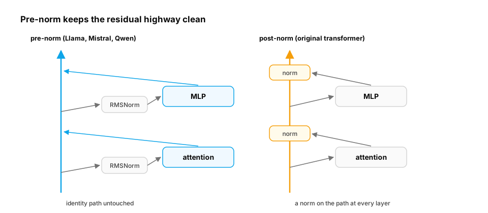
Read it as a residual stream: a running vector per position that every sub-layer reads (through a norm) and writes to (by adding). Nothing overwrites the stream; each layer adds a correction. Two choices matter:
- Pre-norm (normalize the input to each sub-layer) rather than the original post-norm (normalize after adding). Pre-norm leaves the identity path untouched from input to output, so gradients reach early layers directly; post-norm puts a normalization on the path of every residual, which makes deep stacks hard to train without careful warmup.
- RMSNorm instead of LayerNorm: divide by the root-mean-square of the vector and apply a learned scale, without subtracting the mean. Slightly cheaper, and works as well in practice.
import torch
from torch import nn

class RMSNorm(nn.Module):
    def __init__(self, d, eps=1e-6):
        super().__init__(); self.w = nn.Parameter(torch.ones(d)); self.eps = eps
    def forward(self, x):
        return x * torch.rsqrt(x.pow(2).mean(-1, keepdim=True) + self.eps) * self.w

class Sublayer(nn.Module):                               # a stand-in for attention or the MLP
    def __init__(self, d):
        super().__init__(); self.f = nn.Sequential(nn.Linear(d, d), nn.GELU(), nn.Linear(d, d))
    def forward(self, x):
        return self.f(x)

def output_vs_input(depth, pre_norm, d=64):
    fs = [Sublayer(d) for _ in range(depth)]; ns = [RMSNorm(d) for _ in range(depth)]
    x = torch.randn(16, d); h = x
    for f, n in zip(fs, ns):
        h = h + f(n(h)) if pre_norm else n(h + f(h))     # pre-norm: norm inside the branch; post-norm: on the stream
    return nn.functional.cosine_similarity(h, x, dim=-1).mean().item()

torch.manual_seed(0)
with torch.no_grad():
    for depth in [6, 48, 192]:
        pre, post = output_vs_input(depth, True), output_vs_input(depth, False)
        print(f"depth {depth:>3}: how much the output still points along the input (cosine)  pre-norm {pre:.3f}  post-norm {post:.3f}")
The cosine measures how much of the input survives as a direct path to the output. In the pre-norm stack, the input is still clearly present after 192 layers, because every layer only adds to it. In the post-norm stack, each layer's normalization rescales and mixes the whole stream, and by 192 layers the input direction is nearly gone (0.37 against 0.06). The same path carries gradients backwards: with pre-norm, early layers always get a direct route to the loss; with post-norm they depend on gradients passing through every normalization above them, which is why post-norm models need long learning-rate warmup and become unstable as they get deeper (Xiong et al., 2020). At initialization the gradient sizes look similar; the difference shows up during training.
In production. Every widely used open model family (GPT-NeoX, Llama, Mistral, Qwen, Gemma) uses pre-norm, most with RMSNorm. Some add an extra norm after each sub-layer as well ("sandwich" norm, used in Gemma 2) for stability at scale.
Practice.
- Keep the residual path free: no normalization, dropout or scaling directly on the stream, only inside branches.
- Put a final norm after the last block (before the LM head): with pre-norm, nothing else normalizes the stream's output.
- Keep the norm's epsilon and computation in float32 even in mixed precision.
When it breaks. Forgetting the final norm in a pre-norm model trains, but slowly and with poorly scaled logits; removing a residual connection (x = f(n(x)) instead of x = x + f(n(x))) in one layer turns a deep model into one that barely trains. Both show up as loss curves far above a reference implementation's at the same step.
Quick check
Why do modern LLMs use pre-norm blocks rather than the original post-norm arrangement?
Show the answer
B. Pre-norm keeps the residual identity path free of normalization, so gradients reach early layers undiminished and deep stacks train stably without delicate warmup — Each normalization on the residual path rescales gradients; with dozens of layers, post-norm weakens the signal to early layers, while pre-norm's untouched identity path preserves it.
2. The MLP: gated, wide, and where the parameters live
The question. The MLP processes each position on its own. What does it do, and why the strange 8/3 width in Llama-style models?
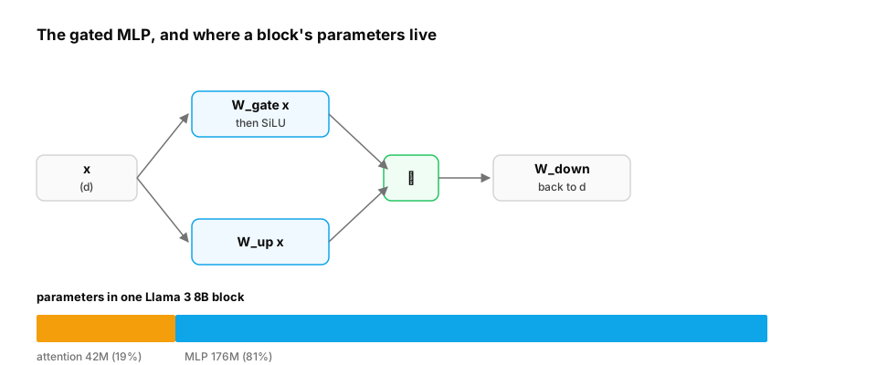
Start from nothing. The classic MLP is W₂ · GELU(W₁ x) with a hidden width of 4d: expand, apply a nonlinearity, project back. One useful mental model is a key–value memory: rows of W₁ act as keys matched against the input, and the corresponding columns of W₂ are the values written back to the stream. Gated MLPs add a third matrix: W₂ · (SiLU(W_gate x) ⊙ W_up x). One branch decides, element by element, how much of the other passes through. At the same compute, SwiGLU trains to a lower loss (Shazeer, 2020). Three matrices instead of two would add 50% more parameters, so Llama-style models shrink the hidden width to about (8/3)·d, rounded to a hardware-friendly multiple, which keeps the parameter count of a 4d GELU MLP.
import torch
from torch import nn

class SwiGLU(nn.Module):
    def __init__(self, d, hidden):
        super().__init__()
        self.gate, self.up = nn.Linear(d, hidden, bias=False), nn.Linear(d, hidden, bias=False)
        self.down = nn.Linear(hidden, d, bias=False)
    def forward(self, x):
        return self.down(nn.functional.silu(self.gate(x)) * self.up(x))

count = lambda m: sum(p.numel() for p in m.parameters())
d = 4096
gelu = nn.Sequential(nn.Linear(d, 4 * d, bias=False), nn.GELU(), nn.Linear(4 * d, d, bias=False))
swiglu = SwiGLU(d, 14336)                                   # Llama 3 8B's MLP width: 3.5 d, a multiple of 1024
print(f"GELU MLP (4d hidden):        {count(gelu) / 1e6:6.1f} M parameters")
print(f"SwiGLU (8/3 d would be 10923; Llama 3 uses 14336): {count(swiglu) / 1e6:6.1f} M parameters")
attn = 2 * d * d + 2 * d * 1024                             # q and o: d x d; k and v: d x (8 KV heads x 128)
print(f"attention with GQA: {attn / 1e6:.1f} M -> MLP share of the block: {count(swiglu) / (count(swiglu) + attn):.0%}")
Llama 3 8B goes further than parameter-matching: its MLP width of 14,336 (3.5 d) makes the MLP about 81% of each block's parameters, because GQA has already made attention cheap. Where parameters live decides where compute and memory go, and which layers matter most for LoRA, quantization and pruning.
In production. Mixture-of-experts models (Mixtral, DeepSeek, Qwen-MoE) replace this one MLP with many expert MLPs and a router that sends each token to a few of them (Architecture families): the MLP is where capacity is cheapest to add.
Practice.
- Round hidden widths to multiples of 64–256 (or the tensor-core tile size); odd widths waste GPU throughput.
- Fuse the gate and up projections into one matrix multiply (
[W_gate; W_up]), as inference engines do. - When fine-tuning with LoRA, include the MLP projections, not only attention: that's where most of the parameters, and much of the knowledge, sit.
When it breaks. Swapping the gate and up weights when converting a checkpoint (SiLU(up) * gate instead of SiLU(gate) * up) gives a model that runs and produces plausible-looking but degraded text; as with GQA head order, a logit comparison against the reference implementation on one prompt catches it.
Quick check
Why do Llama-style SwiGLU MLPs use a hidden width around (8/3)·d instead of 4d?
Show the answer
B. SwiGLU has three weight matrices instead of two; shrinking the width to about 8/3 d keeps the parameter count (and compute) equal to a 4d two-matrix MLP — 3 × d × (8/3)d = 8d² = 2 × d × 4d, so the gated MLP matches the classic one's size while training better at the same compute.
3. The arithmetic: parameters, FLOPs and memory from a config
The question. Given a model's config, how many parameters does it have, how much compute does a token cost, and how much memory does serving or training need?
Start from nothing. Count each matrix:
- Embedding V·d, plus an LM head of the same size unless weights are tied.
- Attention per layer: queries and output d·d each; keys and values d·(kv_heads·d_h) each.
- MLP per layer: 3·d·d_ff for SwiGLU.
- Norms add a negligible 2d per layer.
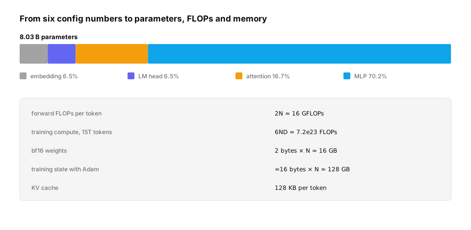
Compute: a forward pass costs about 2 FLOPs per parameter per token (one multiply and one add per weight), plus attention's score computation, about 2·layers·T·d per token, which matters only at long context. A training step (forward plus backward) costs about 6 FLOPs per parameter per token, so a full training run is about 6·N·D FLOPs for N parameters and D tokens.
Memory: weights at 2 bytes per parameter in bf16; training with Adam needs roughly 16 bytes per parameter (weights, gradients, two optimizer moments, an fp32 master copy) before activations (D15).
cfg = dict(vocab=128_256, d=4096, layers=32, heads=32, kv_heads=8, d_ff=14_336, tied=False)   # Llama 3 8B config.json

def count_params(c):
    dh = c["d"] // c["heads"]
    emb = c["vocab"] * c["d"]
    head = 0 if c["tied"] else emb
    attn = 2 * c["d"] * c["d"] + 2 * c["d"] * c["kv_heads"] * dh
    mlp = 3 * c["d"] * c["d_ff"]
    norms = 2 * c["d"]
    return {"embedding": emb, "lm head": head, "attention": c["layers"] * attn, "mlp": c["layers"] * mlp,
            "norms": c["layers"] * norms + c["d"]}

p = count_params(cfg)
N = sum(p.values())
print(f"total {N / 1e9:.2f} B parameters")
for k, v in p.items():
    print(f"   {k:<10} {v / 1e9:5.2f} B ({v / N:5.1%})")
print(f"forward cost ~ {2 * N / 1e9:.0f} GFLOPs per token (+ attention scores: {2 * cfg['layers'] * 8192 * cfg['d'] / 1e9:.1f} GFLOPs/token at 8K context)")
tokens = 15e12
print(f"training on 15T tokens ~ 6 N D = {6 * N * tokens:.2e} FLOPs "
      f"= {6 * N * tokens / (1000 * 400e12 * 0.4) / 86400:.0f} days on 1,000 GPUs at 400 TFLOP/s and 40% utilization")
print(f"memory: bf16 weights {2 * N / 1e9:.0f} GB; full training state with Adam ~ {16 * N / 1e9:.0f} GB before activations")
The count reproduces the published 8.03B parameters exactly, and shows that 13% of a smallish model is embedding and output matrices when the vocabulary is large (a much smaller share in a 70B model), while the MLPs hold 70%. The same six numbers give the compute and memory budget: about 16 GFLOPs per generated token, 16 GB of weights in bf16, and a training run whose cost you can estimate before booking a single GPU.
In production. These are the first calculations in any capacity plan or training proposal. Published scaling-law and cost analyses (Kaplan et al., Chinchilla, the Llama 3 paper) use exactly the 6ND approximation; inference teams use 2N FLOPs per token for prefill throughput and memory bandwidth divided by bytes read per token for decode speed (D12).
Practice.
- Write the parameter count as code next to the model and check it against the instantiated model in a test: it catches wrong widths and accidental untying.
- Quote compute in FLOPs per token and memory in bytes per parameter; both convert directly into GPU-hours and GPUs.
- Remember the KV cache (Lesson I) on top of weights when sizing inference memory.
When it breaks. A plan that sizes inference by weights alone fails in production at long context, when the KV cache, not the weights, exhausts memory; a training budget that ignores activation memory fails at the first long-sequence batch. Both are arithmetic mistakes made before any code runs.
Quick check
Roughly how many FLOPs does it take to train a 7B-parameter model on 2 trillion tokens?
Show the answer
B. About 8.4e22 (6 N D) — Forward plus backward cost about 6 FLOPs per parameter per token: 6 × 7e9 × 2e12 ≈ 8.4e22.
4. From the last hidden state to text
The question. The final block produces a vector per position. How does it become a word, and how should the next token be chosen?
Start from nothing. After the final norm, the LM head (a d → V linear layer, often tied to the embedding matrix) gives logits, one score per vocabulary token; softmax turns them into probabilities. A decoding strategy then picks a token:
- Greedy: the most likely token. Deterministic, but tends to repeat itself in long outputs.
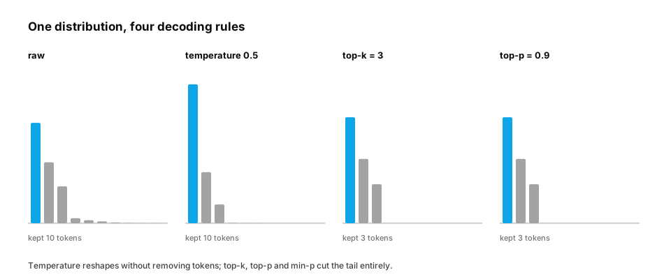
- Temperature: divide logits by T before softmax. T < 1 sharpens, T > 1 flattens.
- Top-k / top-p (nucleus) / min-p: sample only among the k most likely tokens, the smallest set whose probability sums to p, or tokens with at least a fraction of the top token's probability. They cut off the long tail of unlikely tokens that produces nonsense.
- Beam search: keep the b most probable partial sequences. Good for short precise outputs (translation, speech recognition); bland for open-ended text.
import torch

torch.manual_seed(0)
logits = torch.tensor([4.0, 3.5, 3.0, 1.0, 0.5, 0.0, -1.0, -2.0, -2.5, -3.0])

def sample_filter(logits, temperature=1.0, top_k=None, top_p=None, min_p=None):
    z = logits / temperature
    if top_k:
        z = z.masked_fill(z < torch.topk(z, top_k).values[-1], float("-inf"))
    p = torch.softmax(z, -1)
    if top_p:
        sp, idx = p.sort(descending=True)
        keep = sp.cumsum(0) - sp < top_p                       # smallest prefix reaching top_p
        mask = torch.zeros_like(p, dtype=torch.bool); mask[idx[keep]] = True
        p = torch.where(mask, p, torch.zeros_like(p))
    if min_p:
        p = torch.where(p >= min_p * p.max(), p, torch.zeros_like(p))
    return p / p.sum()

for name, kw in [("raw", {}), ("temperature 0.5", {"temperature": 0.5}), ("top-k 3", {"top_k": 3}),
                 ("top-p 0.9", {"top_p": 0.9}), ("min-p 0.1", {"min_p": 0.1})]:
    p = sample_filter(logits, **kw)
    print(f"{name:<16} tokens kept {int((p > 0).sum()):>2}, top token prob {p.max():.2f}, tail (tokens 4+) prob {p[3:].sum():.3f}")
Each strategy reshapes the same distribution differently: temperature changes how peaked it is without removing anything; top-k, top-p and min-p remove the tail entirely, which is what prevents the occasional absurd token in long generations.
In production. Typical settings: temperature 0 (greedy) or low for extraction, classification and tool calling, where determinism and correctness matter; temperature around 0.7–1.0 with top-p 0.9–0.95 for conversation and creative writing. Serving engines apply these per request, and structured-output features constrain sampling further to a grammar or JSON schema (D7).
Practice.
- Make decoding parameters part of each feature's configuration, evaluated like prompts (D7); the same model behaves very differently at temperature 0 and 1.
- For evaluation, fix the sampling settings and seed, or use greedy decoding, so comparisons are reproducible.
- Apply repetition and frequency penalties sparingly; they can distort code and structured output, where repetition is correct.
When it breaks. Endless repetition loops in long greedy outputs ("the the the..." or a repeated paragraph) are the classic greedy failure; the fix is sampling with a modest temperature, a repetition penalty, or a better stopping rule. Rare garbage tokens in long sampled outputs point the other way: the tail isn't being cut (no top-p or min-p).
Quick check
An extraction feature that returns JSON fields sometimes produces different values for the same input. What decoding change is most appropriate?
Show the answer
B. Use greedy decoding (temperature 0) and, where available, schema-constrained output; extraction needs determinism and validity, not diversity — Sampling randomness is useful for open-ended text and harmful for extraction. Greedy plus constrained decoding makes the output deterministic and valid.
5. Numerical stability: keeping large models from diverging
The question. Why do large training runs sometimes spike to NaN after thousands of healthy steps, and what do production models do about it?
Start from nothing. Three sources dominate:
- Low-precision range. fp16's largest value is 65,504; activations or logits above that overflow to infinity. bf16 keeps fp32's range with less precision, which is why it's the default for training. Even so, softmax, norms and the loss should be computed in fp32.
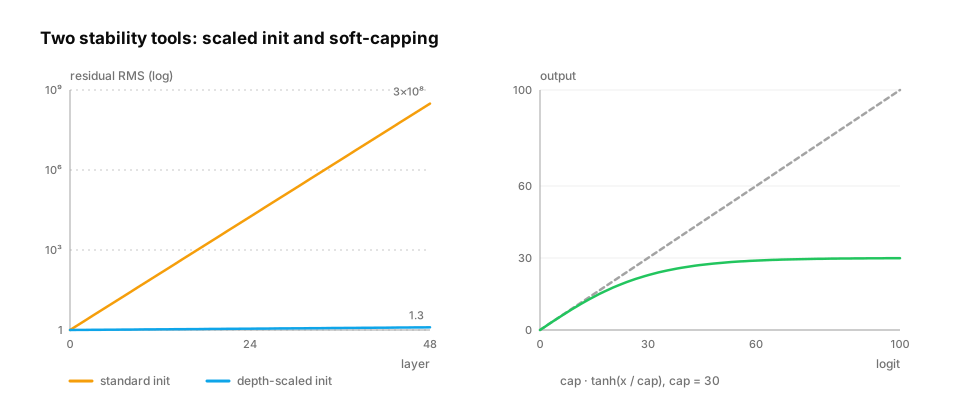
- Growing activations. The residual stream is a sum of every layer's output, so its scale grows with depth unless each branch's output projection is initialized smaller (GPT-2 scales them by 1/√(2·layers)).
- Runaway logits. Attention scores or output logits that drift very large make softmax saturate and gradients explode. Remedies used in published models: z-loss (a small penalty on log of the softmax normalizer, PaLM), QK-norm (normalize queries and keys before the dot product, OLMo 2 and others), and logit soft-capping (
cap · tanh(x / cap), Gemma 2 caps attention logits at 50 and final logits at 30).
import torch

x = torch.tensor([60000.0, 70000.0])
print("fp16 can represent:", x.half().tolist(), "| bf16:", x.bfloat16().tolist())
logits = torch.tensor([12.0, 11.0, 10.0])
naive = lambda z: torch.exp(z) / torch.exp(z).sum()                 # softmax without subtracting the max
print("naive softmax in fp16:", naive(logits.half()).tolist(), "| in fp32:", [round(v, 3) for v in naive(logits).tolist()])

torch.manual_seed(0)
d, layers = 256, 48
for scaled in [False, True]:
    x = torch.randn(64, d)
    std = (1 / (4 * d)) ** 0.5 / ((2 * layers) ** 0.5 if scaled else 1)
    for _ in range(layers):
        for _branch in range(2):                                # attention and MLP each add to the stream
            W_in, W_out = torch.randn(d, 4 * d) / d ** 0.5, torch.randn(4 * d, d) * std
            x = x + torch.relu(x @ W_in) @ W_out
    print(f"{'depth-scaled' if scaled else 'standard    '} output-projection init: residual stream RMS after {layers} layers = {x.pow(2).mean().sqrt():.3g}")

softcap = lambda z, cap: cap * torch.tanh(z / cap)
print("soft-capped logits (cap 30):", [round(v, 1) for v in softcap(torch.tensor([5.0, 30.0, 100.0, 1000.0]), 30).tolist()])
fp16 turns 70,000 into infinity while bf16 keeps it (rounded to 70,144). A softmax written naively overflows in fp16 at a logit of just 12 (e¹² ≈ 162,755) and returns NaN, which is why real kernels subtract the maximum first and accumulate in fp32. With standard initialization, 96 residual additions grow the stream's RMS from 1 to about 3×10⁸; scaling output projections by 1/√(2·layers) keeps it near 1.3. Soft-capping leaves small logits almost unchanged while bounding huge ones smoothly.
In production. Large runs combine these: bf16 mixed precision with fp32 softmax and norms, scaled initialization, gradient clipping (typically at norm 1.0), learning-rate warmup, and one or more of z-loss, QK-norm or soft-capping. Training dashboards track loss, gradient norm and the maximum attention logit per layer, because a growing maximum logit warns of a spike hours before it happens.
Practice.
- Train in bf16, keep fp32 master weights and fp32 reductions (softmax, norms, loss).
- Log gradient norms and max logits per layer, not just the loss.
- When a run spikes, roll back to a checkpoint before the spike, skip the offending data batch, lower the learning rate or add QK-norm, rather than continuing through it.
When it breaks. A loss that is healthy for tens of thousands of steps and then jumps to NaN is the classic large-scale failure. The usual chain: attention logits in a few heads grow, softmax saturates, gradients explode, Adam's update blows up the weights. The gradient-norm and max-logit logs show which layer started it.
Quick check
Why is bf16 preferred over fp16 for training large models, even though both use 16 bits?
Show the answer
B. bf16 keeps fp32's exponent range (no overflow at 65,504), trading precision for range; overflow, not precision, is what destroys training runs — Activations and logits occasionally exceed fp16's maximum and become infinity; bf16's wider range avoids that without loss scaling, at a precision cost training tolerates well.
6. Testing and debugging a transformer
The question. How do you know a new or modified transformer implementation is correct before spending days training it?
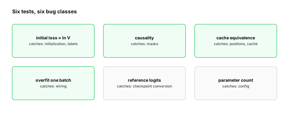
Start from nothing. Most bugs are silent: the code runs, the loss decreases, and the model is subtly wrong. A short test suite catches nearly all of them:
- Initial loss ≈ ln V with a sensible initialization.
- Causality: changing token t never changes outputs at positions < t.
- Cache equivalence: cached decoding matches a full forward pass (Lesson I's exercise).
- Overfit one batch: the model drives the loss on a handful of sequences close to zero.
- Reference equivalence: logits match a trusted implementation on a fixed prompt (when porting or converting checkpoints).
- Parameter count matches the formula from section 3.
import math
import torch
from torch import nn
import torch.nn.functional as F

class TinyLM(nn.Module):
    def __init__(self, V=64, d=64, L=2, h=4):
        super().__init__()
        self.emb = nn.Embedding(V, d); nn.init.normal_(self.emb.weight, std=0.02)
        self.blocks = nn.ModuleList(nn.TransformerEncoderLayer(d, h, 4 * d, dropout=0.0, batch_first=True, norm_first=True) for _ in range(L))
        self.norm, self.head = nn.LayerNorm(d), nn.Linear(d, V, bias=False)
        self.head.weight = self.emb.weight
    def forward(self, ids):
        T = ids.shape[1]; x = self.emb(ids)
        mask = nn.Transformer.generate_square_subsequent_mask(T)
        for b in self.blocks:
            x = b(x, src_mask=mask, is_causal=True)
        return self.head(self.norm(x))

torch.manual_seed(0)
V = 64
m = TinyLM(V)
ids = torch.randint(0, V, (4, 16))
loss_of = lambda m, ids: F.cross_entropy(m(ids)[:, :-1].reshape(-1, V), ids[:, 1:].reshape(-1))

results = {}
results["initial loss near ln V"] = abs(loss_of(m, ids).item() - math.log(V)) < 0.5
ids2 = ids.clone(); ids2[:, 10] = (ids2[:, 10] + 1) % V
m.eval(); results["causal"] = torch.allclose(m(ids)[:, :10], m(ids2)[:, :10], atol=1e-5); m.train()
opt = torch.optim.AdamW(m.parameters(), lr=3e-3)
for step in range(300):
    loss = loss_of(m, ids); opt.zero_grad(); loss.backward(); opt.step()
results["overfits one batch"] = loss.item() < 0.1
d, L = 64, 2                                                  # per layer: qkv + out (4d² + 4d), MLP (8d² + 5d), 2 norms (4d)
results["parameter count"] = sum(p.numel() for p in m.parameters()) == V * d + L * (12 * d * d + 13 * d) + 2 * d
for name, ok in results.items():
    print(f"{'PASS' if ok else 'FAIL'}  {name}")
print(f"final loss on the memorized batch: {loss.item():.4f}")
All checks pass for the correct model, and each check exists because it fails for a specific, common bug: a model that can't overfit 4 sequences has broken wiring, a causality failure is a mask bug, and an initial loss far from ln V is an initialization or label problem. Running the suite takes seconds; skipping it can cost a week of training.
In production. Model repositories (Hugging Face Transformers, Megatron, torchtitan) run tests of exactly these kinds in CI for every architecture, plus numerical comparisons against reference checkpoints; teams porting a model to a new inference engine compare logits layer by layer until they agree to within a small tolerance.
Practice.
- Run the suite in CI on a tiny configuration of your real architecture, not on a toy model.
- Compare against a reference implementation layer by layer when numbers disagree: the first layer that differs locates the bug.
- Keep a fixed "golden" prompt and its expected logits for every released checkpoint.
When it breaks. If a model passes every test here but still behaves oddly, look at the data pipeline next: tokenizer mismatches between training and serving, missing end-of-sequence tokens, and wrong chat templates cause most of the remaining "the model is weird" reports.
Quick check
A refactored transformer trains, but its loss is consistently higher than before the refactor. Which test is the fastest way to locate the problem?
Show the answer
B. Compare logits with the previous implementation layer by layer on a fixed input; the first layer whose outputs differ contains the change that broke it — Layer-by-layer reference comparison turns a vague quality regression into a pinpointed difference, usually a swapped weight, a missing residual or a changed norm.
Check yourself
- What is the residual stream, and why does pre-norm train more stably than post-norm?
- Why is the SwiGLU hidden width about (8/3)·d, and where do most of a block's parameters sit?
- Estimate the parameters, forward FLOPs per token and training FLOPs for a model from its config.
- How do temperature, top-k, top-p and min-p each change the next-token distribution?
- Name three numerical-stability techniques used in production LLMs and what each prevents.
- List four tests every transformer implementation should pass and the bug each catches.
Answers
- A per-position vector that each sub-layer reads through a norm and adds to. Pre-norm keeps the identity path free of normalization, so gradients reach early layers undiminished.
- Three matrices instead of two; 8/3 width keeps parameters equal to a 4d MLP. In the MLP (two thirds or more of each block).
- Embedding V·d (twice if untied) + layers × (2d² + 2·d·kv·d_h + 3·d·d_ff); forward ≈ 2N FLOPs per token; training ≈ 6·N·D.
- Temperature rescales peakedness without removing tokens; top-k keeps the k most likely; top-p keeps the smallest set reaching probability p; min-p keeps tokens with at least a fraction of the top probability.
- bf16 with fp32 reductions (overflow), depth-scaled initialization (residual growth), z-loss/QK-norm/soft-capping (runaway logits); gradient clipping and warmup (update blow-ups).
- Initial loss ≈ ln V (initialization/labels), causality (masks), cache equivalence (positions/cache), overfit one batch (wiring), reference logits (conversion), parameter count (config).
Exercise
Write a config-to-budget tool: given a Hugging Face–style config (vocab size, hidden size, layers, heads, KV heads, MLP width, tied embeddings), print the parameter count by component, bf16 weight memory, KV-cache bytes per token, the maximum number of concurrent 8K-token sequences on an 80 GB GPU after weights, and the 6ND training compute for a token budget. Run it for Llama 3 8B and for a 70B configuration (80 layers, d 8192, 64 heads, 8 KV heads, d_ff 28,672, vocab 128,256), and explain what limits each.
Solution
def budget(name, vocab, d, layers, heads, kv_heads, d_ff, tied=False, train_tokens=15e12, gpu_gb=80, ctx=8192):
    dh = d // heads
    emb = vocab * d
    per_layer = 2 * d * d + 2 * d * kv_heads * dh + 3 * d * d_ff + 2 * d
    N = emb * (1 if tied else 2) + layers * per_layer + d
    weights_gb = 2 * N / 1e9
    kv_per_token = 2 * layers * kv_heads * dh * 2                   # bytes, bf16
    free_gb = gpu_gb - weights_gb
    seqs = int(free_gb * 1e9 // (kv_per_token * ctx)) if free_gb > 0 else 0
    print(f"{name}: {N / 1e9:.2f} B params, weights {weights_gb:.0f} GB, KV {kv_per_token / 1024:.0f} KB/token")
    if free_gb > 0:
        print(f"   one 80 GB GPU: {free_gb:.0f} GB left after weights -> {seqs} concurrent {ctx}-token sequences")
    else:
        print(f"   weights alone need {weights_gb / gpu_gb:.1f} GPUs: shard with tensor parallelism (D15)")
    print(f"   training on {train_tokens / 1e12:.0f}T tokens: {6 * N * train_tokens:.2e} FLOPs")

budget("Llama 3 8B", 128_256, 4096, 32, 32, 8, 14_336)
budget("70B-class", 128_256, 8192, 80, 64, 8, 28_672)
The 8B model fits on one GPU with room for a few dozen concurrent 8K-token conversations, so its limit is KV-cache memory per user. The 70B model's weights alone exceed one 80 GB GPU, so it must be sharded across GPUs before the question of concurrency even arises, and its KV cache per token is 2.5× larger than the 8B's despite having the same number of KV heads, because it has more layers. These are the first numbers in any serving or training plan, and they come straight from the config.
This unlocks:
- Architecture families — MoE, state-space and hybrid alternatives to this block.
- LLM pretraining — the data, compute and scaling laws behind training it.
- Inference fundamentals (D12) — prefill, decode and the costs computed here.
Sources: Xiong et al., On Layer Normalization in the Transformer Architecture (2020); Zhang & Sennrich, Root Mean Square Layer Normalization (2019); Shazeer, GLU Variants Improve Transformer (2020); Geva et al., Transformer Feed-Forward Layers Are Key-Value Memories (2021); Kaplan et al., Scaling Laws for Neural Language Models (2020); Radford et al., Language Models are Unsupervised Multitask Learners (GPT-2, scaled init, 2019); Chowdhery et al., PaLM (z-loss, 2022); Gemma Team, Gemma 2 (soft-capping, 2024); OLMo Team, 2 OLMo 2 Furious (QK-norm, 2024); Holtzman et al., The Curious Case of Neural Text Degeneration (top-p, 2020); Nguyen et al., Min-p sampling (2024); Meta, The Llama 3 Herd of Models (2024).