You already know: tokens and embeddings (NLP foundations); matrix multiplication and the dot product (D2 Linear algebra); softmax and probabilities (D2 Probability); residual connections and normalization (D4 Fundamentals).
Why this matters for Atlas. Every modern language model, from a 1M-parameter TinyGPT to the frontier, is the same stack: embeddings, then N identical blocks of attention and MLP, then a projection back to the vocabulary. This module takes it apart in two lessons. This lesson builds the attention side from first principles: the shapes of the whole forward pass, why attention is a scaled dot product, how position gets in (RoPE and long context), and why modern models share keys and values across heads (MQA, GQA, MLA). Lesson II (The Transformer II) covers the block, the output layer, parameter and FLOP accounting, and the numerical and engineering practices production models depend on.
Where you'll use this. Reading a model card or
config.jsonand knowing what each number costs (an inference team sizing GPUs for a new open model). Debugging a fine-tune whose loss is fine but whose generations go wrong after a few hundred tokens (almost always positions or masks). Choosing between two models of the same size for a long-context product, where the KV-cache cost of their attention variants differs by 8×.
1. The whole forward pass on one page
The question. Before any detail: what exactly goes in, what comes out, and what shape is every tensor along the way?
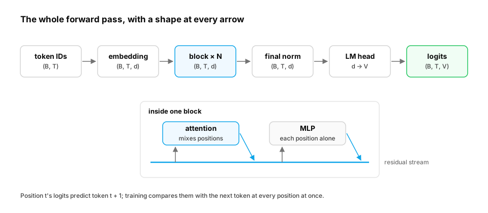
Start from nothing. A decoder-only transformer maps a batch of token IDs to a score for every possible next token, at every position:
- Input: integer IDs of shape
(B, T): B sequences of T tokens. - Embedding: look up a row of a
(V, d)matrix for each ID →(B, T, d), where V is the vocabulary size and d the model width. - N blocks: each block keeps the shape
(B, T, d). Inside, attention mixes information across positions; the MLP transforms each position independently. Both add their result back onto the input (the residual stream). - Output: a final normalization, then the LM head (a
(d, V)matrix, often the transpose of the embedding) gives logits(B, T, V). Position t's logits are the model's prediction for token t + 1.
Training uses all T predictions at once (teacher forcing: every position predicts its next token in parallel). Generation uses only the last position's logits, samples a token, appends it and repeats.
import torch
from torch import nn

B, T, V, d, N = 2, 8, 1000, 64, 3
ids = torch.randint(0, V, (B, T))
emb = nn.Embedding(V, d)
nn.init.normal_(emb.weight, std=0.02)                          # small init: N(0, 1) embeddings would give huge tied logits
blocks = nn.ModuleList(nn.TransformerEncoderLayer(d, 4, 4 * d, batch_first=True, norm_first=True) for _ in range(N))
head = nn.Linear(d, V, bias=False)
head.weight = emb.weight                                       # weight tying: one (V, d) matrix at both ends

x = emb(ids)
print(f"ids {tuple(ids.shape)} -> embeddings {tuple(x.shape)}")
mask = nn.Transformer.generate_square_subsequent_mask(T)
for i, blk in enumerate(blocks):
    x = blk(x, src_mask=mask, is_causal=True)
    print(f"after block {i}: {tuple(x.shape)}")
logits = head(x)
print(f"logits {tuple(logits.shape)}  (position t scores every vocabulary token as the next one)")
targets = torch.roll(ids, -1, dims=1)                          # next-token targets: shift left by one
loss = nn.functional.cross_entropy(logits[:, :-1].reshape(-1, V), targets[:, :-1].reshape(-1))
print(f"initial loss {loss.item():.2f} vs ln(V) = {torch.log(torch.tensor(float(V))).item():.2f} (uniform guessing)")
The initial loss sits near ln V, the loss of guessing uniformly over the vocabulary, a quick sanity check that the pipeline is wired correctly before any training. (Leave the embedding at PyTorch's default N(0, 1) initialization and the tied LM head produces huge logits: the loss starts around 67, ten times ln V, a typical symptom of an initialization mistake.)
In production. A model's config.json is this page in numbers. Llama 3 8B, for example, has 32 layers, d = 4,096, 32 query heads, 8 key/value heads, an MLP width of 14,336 and a vocabulary of 128,256 tokens; reading those six numbers tells you its parameter count, its KV-cache cost per token and roughly how fast it can decode (Lesson II does the arithmetic).
Practice.
- Write the shape of every tensor in a comment, and
assertshapes at module boundaries; most transformer bugs are silent shape or axis mistakes. - Check the initial loss against ln V before training anything: far above it means bad initialization; far below means labels are leaking into inputs.
- Keep "predict t + 1 from ≤ t" explicit in the code that builds targets: the shift is a classic off-by-one.
When it breaks. A loss that drops to almost zero within a few steps usually means the model can see the answer: the targets weren't shifted, or the causal mask is missing, so position t reads token t + 1 directly.
Quick check
A new training script's loss falls from 7.0 to 0.05 in 200 steps on a large, varied corpus. What's the most likely explanation?
Show the answer
B. The model can see the token it's predicting: targets not shifted by one, or the causal mask is missing — Near-zero loss on real text this fast means information about the target leaks into the input. Check the target shift and the mask before celebrating.
2. Attention from first principles
The question. Each position needs information from earlier positions, but which ones, and how much? Why does the formula end up as softmax(QKᵀ/√d)V?
Start from nothing. Give every position three vectors, each a learned linear projection of its residual-stream vector:
- a query q: what this position is looking for;
- a key k: what this position offers for others to match against;
- a value v: the information it passes on if chosen.
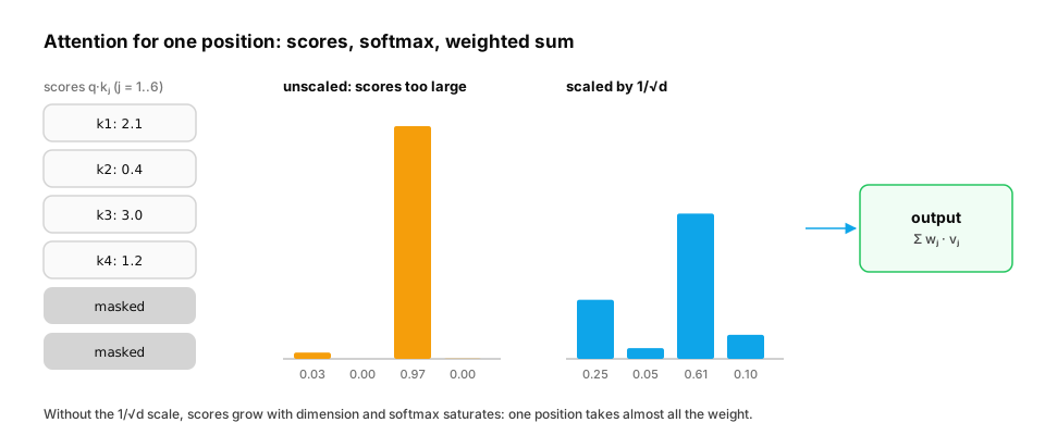
Relevance between position i (asking) and j (offering) is the dot product qᵢ·kⱼ: large when the two vectors point the same way. A softmax over j turns the scores into weights that are positive and sum to 1, and position i's output is the weighted average of the values. A causal mask sets the scores for j > i to −∞, so their weights are exactly 0: no peeking at the future.
Why divide by √d? If q and k have independent components with unit variance, their dot product is a sum of d products, so its variance is d. With d = 128, scores have a standard deviation of about 11, and softmax over such large numbers becomes nearly one-hot: one position takes almost all the weight, and gradients through the others vanish. Dividing by √d brings the variance back to about 1.
import math
import torch
import torch.nn.functional as F

torch.manual_seed(0)
for d in [16, 128, 1024]:
    q, k = torch.randn(10_000, d), torch.randn(10_000, d)
    raw = (q * k).sum(-1)
    print(f"d = {d:>4}: std of q.k = {raw.std():6.2f} (sqrt(d) = {math.sqrt(d):5.2f}); after / sqrt(d): {(raw / math.sqrt(d)).std():.2f}")

d, T = 128, 6
q, k = torch.randn(T, d), torch.randn(T, d)
raw_w = torch.softmax(q[-1] @ k.T, -1)
scaled_w = torch.softmax(q[-1] @ k.T / math.sqrt(d), -1)
print("largest weight without scaling:", round(raw_w.max().item(), 3), "| with scaling:", round(scaled_w.max().item(), 3))

def attention(q, k, v):                                        # (B, h, T, dh): attention from scratch
    T, dh = q.shape[-2], q.shape[-1]
    scores = q @ k.transpose(-2, -1) / math.sqrt(dh)
    future = torch.triu(torch.ones(T, T, dtype=torch.bool), diagonal=1)
    scores = scores.masked_fill(future, float("-inf"))
    return torch.softmax(scores, dim=-1) @ v

q, k, v = torch.randn(3, 2, 4, 6, 32).unbind(0)
ours = attention(q, k, v)
ref = F.scaled_dot_product_attention(q, k, v, is_causal=True)
print("matches PyTorch's fused kernel:", torch.allclose(ours, ref, atol=1e-5))
The spread of raw dot products grows as √d, scaling restores it to about 1, and without scaling one key soaks up nearly all the weight. The 10-line version matches PyTorch's fused scaled_dot_product_attention exactly.
In production. Nobody materializes the T × T score matrix at scale: fused kernels (FlashAttention, PyTorch SDPA, cuDNN attention) compute the same result tile by tile in on-chip memory, turning attention's memory cost from quadratic to linear in T (D13). The maths in this section is exactly what they compute; only the order of operations changes.
Practice.
- Call the fused kernel (
F.scaled_dot_product_attention) in real code, and keep a from-scratch version in tests to check it against. - Compute softmax in float32 even when the model runs in bfloat16; large logits in low precision overflow or lose the small weights.
- Use the
is_causalflag or a boolean mask rather than adding large negative numbers by hand, which behave differently in fp16 and fp32.
When it breaks. Two real bugs. First, mask conventions differ between APIs: in nn.MultiheadAttention a boolean mask's True means blocked, while in F.scaled_dot_product_attention True means allowed. Porting code between them silently inverts the mask. Second, a row whose positions are all masked (a padding-only row) has no valid weights at all: a hand-written softmax over all −∞ gives NaN, which then spreads through the batch, while recent fused kernels return zeros, which is quieter and therefore harder to notice.
import torch
import torch.nn.functional as F

T = 4
causal_blocked = torch.triu(torch.ones(T, T, dtype=torch.bool), diagonal=1)   # True = "blocked" (nn.MultiheadAttention style)
q = k = v = torch.randn(1, 1, T, 8)
right = F.scaled_dot_product_attention(q, k, v, attn_mask=~causal_blocked)    # SDPA wants True = "allowed"
wrong = F.scaled_dot_product_attention(q, k, v, attn_mask=causal_blocked)     # the ported mask, unconverted
print("correct mask matches is_causal:", torch.allclose(right, F.scaled_dot_product_attention(q, k, v, is_causal=True)))
print("unconverted mask, last position via SDPA:", wrong[0, 0, -1, :3].tolist(), "(silently zero in recent PyTorch)")
scores = (q @ k.transpose(-2, -1)).masked_fill(~causal_blocked, float("-inf"))      # same mistake, hand-written
print("same row with a hand-written softmax:", torch.softmax(scores, -1)[0, 0, -1, :3].tolist())
print("unconverted mask, first position attends to:", (~causal_blocked[0]).logical_not().nonzero().flatten().tolist(), "(only the future)")
The unconverted mask lets every position see only the future, and the last position, which has no future, can attend to nothing at all. The fused kernel silently returns zeros for it; the hand-written softmax returns NaN. Neither raises an error, which is why mask bugs survive until someone checks outputs against a reference.
Quick check
Why are attention scores divided by √d_head?
Show the answer
B. Dot products of d-dimensional vectors with unit-variance components have variance about d; dividing by √d keeps scores near unit scale so softmax isn't pushed into a near one-hot, gradient-starved regime — Without scaling, wider heads produce larger scores and a saturated softmax; scaling keeps the attention distribution trainable at any head size.
3. Position: from sinusoids to RoPE and long context
The question. Attention as written is a weighted average over a set: shuffle the tokens and every output is shuffled the same way. How does the model tell "dog bites man" from "man bites dog"?
Start from nothing. Position must be injected. The options, in historical order:
- Sinusoidal absolute positions (original transformer): add fixed sine/cosine waves of different frequencies to each embedding.
- Learned absolute positions (GPT-2, BERT): a trainable vector per position; simple, but undefined beyond the trained length.
- Relative biases (T5, ALiBi): add a term to the attention score that depends on the distance i − j.
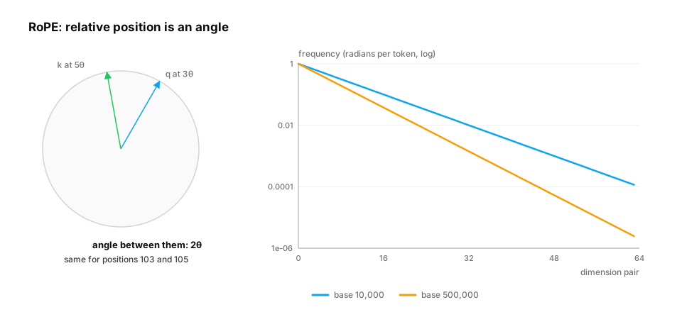
- Rotary position embeddings (RoPE) (LLaMA, Mistral, Qwen and most current models): rotate each pair of dimensions of q and k by an angle proportional to the position, with a different frequency per pair. Rotating q by mθ and k by nθ makes their dot product depend only on (m − n)θ: attention sees relative distance, while each vector is processed with its absolute position, which keeps it compatible with the KV cache.
Long context. A model trained on 8K tokens has never seen the rotation angles of position 100K for its low-frequency pairs. Position interpolation squeezes new positions into the trained range (divide positions by the extension factor); NTK-aware scaling and YaRN instead raise the RoPE base (θ), stretching low frequencies a lot and high frequencies little, so local word order stays sharp while long distances become representable. This is why long-context variants of a model mostly differ in one config field (rope_theta or rope_scaling) plus a short fine-tune at the new length.
import torch

def rope(x, positions, base=10000.0):
    """x: (seq, dim), dim even. Rotate each (even, odd) pair by position x frequency."""
    d = x.shape[-1]
    freqs = base ** (-torch.arange(0, d, 2, dtype=torch.float32) / d)
    angles = positions[:, None].float() * freqs[None, :]
    cos, sin = angles.cos(), angles.sin()
    x1, x2 = x[..., 0::2], x[..., 1::2]
    out = torch.empty_like(x)
    out[..., 0::2] = x1 * cos - x2 * sin
    out[..., 1::2] = x1 * sin + x2 * cos
    return out

torch.manual_seed(0)
q, k = torch.randn(1, 64), torch.randn(1, 64)
score = lambda m, n, base=10000.0: (rope(q, torch.tensor([m]), base) @ rope(k, torch.tensor([n]), base).T).item()
print(f"positions (3, 5): {score(3, 5):.4f}   (103, 105): {score(103, 105):.4f}   <- same distance, same score")
print(f"positions (3, 50): {score(3, 50):.4f}   <- different distance, different score")
print("rotation preserves length:", torch.allclose(rope(q, torch.tensor([7])).norm(), q.norm()))

# Long context: how many full turns the slowest dimension pair makes over a context, for two bases
d = 128
for base in [10_000.0, 500_000.0]:
    slowest = base ** (-(d - 2) / d)                           # frequency of the last pair
    for ctx in [8_192, 131_072]:
        print(f"base {base:>9,.0f}: slowest pair turns {ctx * slowest / (2 * 3.14159):6.2f} times over {ctx:,} tokens")
With base 10,000 the slowest dimension pair turns only 0.15 times across an 8K context, but more than twice across 128K tokens: far-apart positions start to alias with nearer ones, at angles the model never saw in training. Raising the base to 500,000 (Llama 3's value) keeps the slowest pair at a twentieth of a turn even at 128K tokens, which is the headroom long-context models need.
In production. Llama 3 uses rope_theta = 500000; Llama 3.1 adds a rope_scaling entry to reach 128K tokens; Mistral and Qwen ship similar fields. Serving engines must apply exactly the scaling the checkpoint was trained with, which is why loading a long-context model with an older library version can quietly degrade quality beyond the original length.
Practice.
- Treat RoPE settings (
rope_theta,rope_scaling, head dimension) as part of the model, versioned with the weights. - During cached decoding, the new token's position is the number of tokens already in the cache, not 0; get the position IDs from the cache length.
- With left padding (common for batched generation), compute position IDs from the attention mask, not from the raw index.
When it breaks. Generations that are fluent for the first few hundred tokens and then degrade into repetition or nonsense are the signature of a position bug: decoding with positions restarting at 0, padding counted as positions, or the wrong RoPE scaling. The fix is to log the position IDs for one batch and compare them with the training data pipeline.
Quick check
A model fine-tuned at 4K context is served with the original model's RoPE settings, while the fine-tune used rope_scaling for 32K. Outputs are fine for short prompts but degrade on long documents. Why?
Show the answer
B. Positions beyond the original range are rotated with angles the fine-tuned model never saw; the serving config must reproduce the training-time RoPE scaling — RoPE scaling changes the rotation frequencies. Serving with a different setting than training means long-range positions are encoded inconsistently, which shows up only beyond the original length.
4. Heads: multi-head, multi-query, grouped-query and latent attention
The question. Why split attention into many small heads, and why do nearly all modern LLMs share keys and values across those heads?
Start from nothing. Multi-head attention (MHA) splits d into h heads of size d_h = d/h, each with its own q, k and v projections, attending independently; their outputs are concatenated and projected back to d. Same compute as one wide head, but h different attention patterns (one head tracks the previous token, another a matching bracket, another the subject of the sentence).
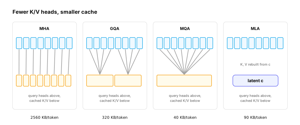
During generation, every past token's keys and values are cached (the KV cache, D12): per token that's 2 × layers × kv_heads × d_h numbers. It grows with every token and every concurrent user, and reading it dominates the time of each decode step. So:
- Multi-query attention (MQA): all query heads share one key/value head. Smallest cache; a measurable quality cost.
- Grouped-query attention (GQA): query heads are split into g groups, each sharing one K/V head (Llama 3 8B: 32 query heads, 8 KV heads). Close to MHA quality at a 4× smaller cache.
- Multi-head latent attention (MLA) (DeepSeek-V2/V3): cache one low-rank latent vector per token (plus a small RoPE part) and reconstruct per-head keys and values from it, shrinking the cache further while keeping per-head expressiveness.
import torch
import torch.nn.functional as F

def gqa_attention(x, Wq, Wk, Wv, n_heads, n_kv_heads):
    B, T, D = x.shape
    dh = D // n_heads
    q = (x @ Wq).view(B, T, n_heads, dh).transpose(1, 2)               # (B, h, T, dh)
    k = (x @ Wk).view(B, T, n_kv_heads, dh).transpose(1, 2)            # (B, kv, T, dh)
    v = (x @ Wv).view(B, T, n_kv_heads, dh).transpose(1, 2)
    group = n_heads // n_kv_heads
    k, v = k.repeat_interleave(group, dim=1), v.repeat_interleave(group, dim=1)   # query head i uses kv head i // group
    return F.scaled_dot_product_attention(q, k, v, is_causal=True).transpose(1, 2).reshape(B, T, D)

torch.manual_seed(0)
B, T, D, H, KV = 2, 6, 64, 8, 2
x = torch.randn(B, T, D)
Wq = torch.randn(D, D) / D ** 0.5
Wk, Wv = torch.randn(D, KV * D // H) / D ** 0.5, torch.randn(D, KV * D // H) / D ** 0.5
out = gqa_attention(x, Wq, Wk, Wv, H, KV)
x2 = x.clone(); x2[:, -1] += 10                                          # change only the last token
print("output", tuple(out.shape), "| earlier positions unaffected by the future:",
      torch.allclose(out[:, :-1], gqa_attention(x2, Wq, Wk, Wv, H, KV)[:, :-1], atol=1e-5))

def kv_bytes_per_token(layers, kv_heads, dh, bytes_per=2):
    return 2 * layers * kv_heads * dh * bytes_per

shape = dict(layers=80, dh=128)                                          # a 70B-class model, bf16
for name, kv in [("MHA (64 KV heads)", 64), ("GQA (8 KV heads)", 8), ("MQA (1 KV head)", 1)]:
    per_tok = kv_bytes_per_token(kv_heads=kv, **shape)
    print(f"{name:<18} {per_tok / 1024:7.0f} KB per token -> {per_tok * 32_768 / 1e9:5.1f} GB for one 32K-token sequence")
mla = 80 * (512 + 64) * 2                                                # latent 512 + RoPE part 64, one per layer
print(f"{'MLA (latent 512+64)':<18} {mla / 1024:7.0f} KB per token -> {mla * 32_768 / 1e9:5.1f} GB")
GQA computes exactly the same kind of causal attention while storing a quarter or less of the keys and values, and the KV-cache table shows why it matters: at a 32K context, full multi-head attention on a 70B-class model needs over 85 GB for one sequence, GQA about 11 GB, and a latent cache less than that.
In production. Published configs show the convergence: Llama 2 70B and Llama 3 use GQA with 8 KV heads; Mistral 7B uses 32 query and 8 KV heads; DeepSeek-V2/V3 use MLA. For an inference team, num_key_value_heads in the config is the single most important number for capacity planning: it sets how many concurrent long conversations fit on a GPU (D12).
Practice.
- Keep
n_heads % n_kv_heads == 0as an assertion; GQA requires query heads to divide evenly into groups. - Use
expand(a view) rather thanrepeat_interleave(a copy) for the K/V broadcast in performance-sensitive code, or rely on kernels that support GQA natively. - When converting checkpoints between frameworks, check the head ordering convention for grouping (interleaved vs blocked) with a numerical test against the reference implementation.
When it breaks. A converted GQA checkpoint that produces fluent but subtly wrong text often has its query heads paired with the wrong KV heads: repeat_interleave (head i → KV head i // group) and tile-style repetition (head i → KV head i % kv) give different, both plausible-looking, models. Comparing logits on a fixed prompt against the original implementation catches it in seconds.
Quick check
Two 70B models have the same quality. One uses 64 KV heads (MHA), the other 8 (GQA). What's the practical serving difference at long context?
Show the answer
B. The GQA model's KV cache is 8x smaller per token, so far more concurrent long conversations fit in GPU memory and each decode step reads less memory, making it faster — KV-cache size scales with the number of KV heads. At long context the cache, not the weights, limits concurrency and decode speed.
Check yourself
- What are the input and output shapes of a decoder-only transformer, and what does position t's output predict?
- Why does the dot product of two random d-dimensional vectors need scaling by 1/√d before softmax?
- What makes RoPE "relative", and what do NTK/YaRN scaling change for long context?
- How large is the KV cache per token, and how do MQA, GQA and MLA reduce it?
- Name one mask bug and one position bug, and the symptom of each.
Answers
(B, T)token IDs in,(B, T, V)logits out; position t's logits score every vocabulary token as token t + 1.- Its variance grows as d, so unscaled scores saturate the softmax into a near one-hot distribution with vanishing gradients; dividing by √d keeps variance near 1.
- Rotating q and k by position-proportional angles makes their dot product depend only on the position difference. NTK/YaRN raise the RoPE base, stretching low frequencies so long distances stay representable while local order stays sharp.
- 2 × layers × kv_heads × d_h × bytes. MQA uses one KV head, GQA one per group of query heads, MLA caches a low-rank latent per token from which keys and values are reconstructed.
- Mask: porting a boolean mask between APIs with opposite conventions (inverted masking, NaNs for rows that can see nothing). Position: restarting positions at 0 during cached decoding (fluent start, degradation after a few hundred tokens).
Exercise
Assemble an attention module you'd be happy to put in a real model: CausalSelfAttention(d_model, n_heads, n_kv_heads, rope_theta) with RoPE applied to queries and keys, grouped-query attention, an optional KV cache, and correct position IDs during cached decoding. Test that (a) cached step-by-step decoding produces the same outputs as one full forward pass, and (b) changing a future token never changes earlier outputs.
Solution
import torch
from torch import nn
import torch.nn.functional as F

def apply_rope(x, positions, theta):                      # x: (B, h, T, dh)
    dh = x.shape[-1]
    freqs = theta ** (-torch.arange(0, dh, 2, dtype=torch.float32) / dh)
    ang = positions[:, None].float() * freqs
    cos, sin = ang.cos(), ang.sin()
    x1, x2 = x[..., 0::2], x[..., 1::2]
    return torch.stack([x1 * cos - x2 * sin, x1 * sin + x2 * cos], dim=-1).flatten(-2)

class CausalSelfAttention(nn.Module):
    def __init__(self, d, h, kv, theta=10000.0):
        super().__init__()
        assert d % h == 0 and h % kv == 0
        self.h, self.kv, self.dh, self.theta = h, kv, d // h, theta
        self.q = nn.Linear(d, d, bias=False)
        self.k = nn.Linear(d, kv * self.dh, bias=False)
        self.v = nn.Linear(d, kv * self.dh, bias=False)
        self.o = nn.Linear(d, d, bias=False)

    def forward(self, x, cache=None):
        B, T, _ = x.shape
        start = 0 if cache is None else cache[0].shape[2]          # positions continue from the cache length
        pos = torch.arange(start, start + T)
        q = apply_rope(self.q(x).view(B, T, self.h, self.dh).transpose(1, 2), pos, self.theta)
        k = apply_rope(self.k(x).view(B, T, self.kv, self.dh).transpose(1, 2), pos, self.theta)
        v = self.v(x).view(B, T, self.kv, self.dh).transpose(1, 2)
        if cache is not None:
            k, v = torch.cat([cache[0], k], 2), torch.cat([cache[1], v], 2)
        g = self.h // self.kv
        kk, vv = k.repeat_interleave(g, 1), v.repeat_interleave(g, 1)
        out = F.scaled_dot_product_attention(q, kk, vv, is_causal=cache is None)   # a single new query may see everything
        return self.o(out.transpose(1, 2).reshape(B, T, -1)), (k, v)

torch.manual_seed(0)
attn = CausalSelfAttention(64, 8, 2).eval()
x = torch.randn(2, 10, 64)
full, _ = attn(x)
outs, cache = [], None
for t in range(10):                                               # token by token, with the cache
    o, cache = attn(x[:, t:t + 1], cache)
    outs.append(o)
print("cached decoding matches the full pass:", torch.allclose(torch.cat(outs, 1), full, atol=1e-5))
x2 = x.clone(); x2[:, -1] += 5
print("causal:", torch.allclose(attn(x2)[0][:, :-1], full[:, :-1], atol=1e-5))
The two tests are the ones production teams run on every new attention implementation: equality between cached and uncached decoding catches position-ID and cache bugs, and the causality test catches mask bugs. The positions in the cached path start from the cache length, which is exactly the bug from section 3 handled correctly.
This unlocks:
- The Transformer II — the block, the output layer, parameter and FLOP accounting, and production practice.
- Architecture families — encoders, encoder–decoders, MoE and state-space alternatives.
- KV cache engineering (D12) — serving the cache this lesson sized.
Sources: Vaswani et al., Attention Is All You Need (2017); Su et al., RoFormer: Rotary Position Embedding (2021); Chen et al., Extending Context Window of LLMs via Positional Interpolation (2023); Peng et al., YaRN (2023); Shazeer, Fast Transformer Decoding: One Write-Head is All You Need (MQA, 2019); Ainslie et al., GQA (2023); DeepSeek-AI, DeepSeek-V2 (MLA, 2024); Dao et al., FlashAttention (2022); Meta, Llama 3 model card and config.json; PyTorch documentation for scaled_dot_product_attention and MultiheadAttention.