Problem. You have a batch X of n feature vectors, each of dimension d (an n × d matrix).
- L2-normalise each row: divide every row by its length, so each has norm 1 (used before cosine similarity).
- Standardise each column: subtract the column mean and divide by the column standard deviation (used before training most models).
X = [[3, 4],          row norms [5, 10]        →   [[0.6, 0.8],
     [6, 8]]                                         [0.6, 0.8]]
This is the module's ML twin: nothing here is an interview puzzle, but every idea from module 01 shows up. Arrays and memory layout (1.1), running sums (1.2), one-pass statistics, and the habit of asking what happens when the constraints change. The complexity barely changes (it's O(n · d) from start to finish); what changes is the constant, numerical stability and correctness in production.
1. Step 1: Clarify
| Question | Answer | Why it matters |
|---|---|---|
| Shape? | n × d, e.g. 10⁵ × 768 | 7.7 × 10⁷ values: Python loops are too slow |
| Can a row be all zeros? | Yes (padding, empty documents) | Division by zero → NaN |
| Can a column be constant? | Yes | Standard deviation 0 → division by zero |
| Does it fit in memory? | Sometimes not | Streaming statistics |
| Training or serving? | Both | Statistics must come from the training data only |
2. Step 2: Brute force: nested Python loops
Compute each row's norm by looping over its values, then divide. Note the hidden waste: this version recomputes the norm for every element.
import math


def l2_normalise_naive(X):
    out = []
    for row in X:
        new_row = []
        for x in row:
            norm = math.sqrt(sum(v * v for v in row))      # recomputed d times per row!
            new_row.append(x / norm)
        out.append(new_row)
    return out


X = [[3.0, 4.0], [6.0, 8.0]]
assert l2_normalise_naive(X) == [[0.6, 0.8], [0.6, 0.8]]
print("naive version works: O(n · d²) time")
O(n · d²): for 10⁵ rows of dimension 768, about 6 × 10¹⁰ operations. The first fix is the same as lesson 1.2's: don't recompute what you can compute once.
3. Step 3: Optimise
Optimisation 1: compute each norm once (O(n · d))
import math


def l2_normalise_loops(X):
    out = []
    for row in X:
        norm = math.sqrt(sum(v * v for v in row))          # once per row: O(d)
        out.append([v / norm for v in row])
    return out


X = [[3.0, 4.0], [6.0, 8.0]]
assert l2_normalise_loops(X) == [[0.6, 0.8], [0.6, 0.8]]
print("one norm per row: O(n · d) time")
Now O(n · d), which is optimal: every value must be read and written. But each step still runs in the Python interpreter, which costs tens of nanoseconds per operation. With 7.7 × 10⁷ values, that's seconds per batch.
Optimisation 2: vectorise with NumPy (same O(n · d), much smaller constant)
First principles (lesson 1.1): a NumPy array is one contiguous buffer, and its operations run as compiled loops.
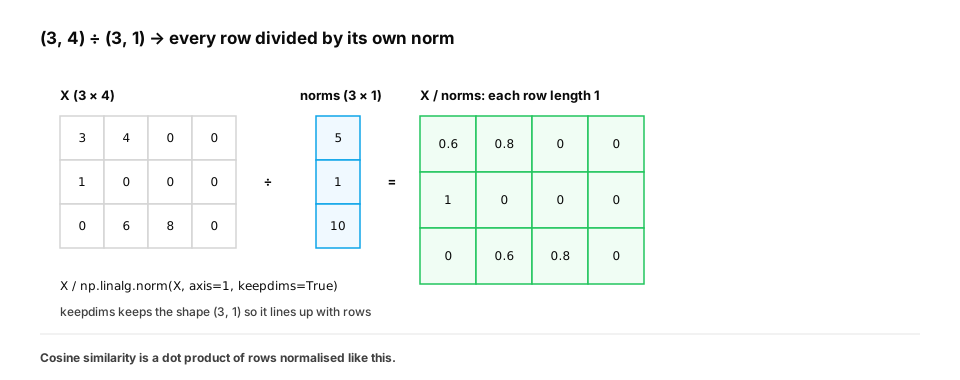
np.linalg.norm(X, axis=1, keepdims=True) computes all row norms at once with shape (n, 1); dividing X (n, d) by
it broadcasts the norm across each row.
import math
import time

import numpy as np


def l2_normalise_loops(X):
    out = []
    for row in X:
        norm = math.sqrt(sum(v * v for v in row))
        out.append([v / norm for v in row])
    return out


def l2_normalise(X):
    return X / np.linalg.norm(X, axis=1, keepdims=True)   # (n, d) / (n, 1)


rng = np.random.default_rng(32)
X = rng.normal(size=(2000, 128))
Y = l2_normalise(X)
assert np.allclose(np.linalg.norm(Y, axis=1), 1.0)
assert np.allclose(Y, np.array(l2_normalise_loops(X.tolist())))

t0 = time.perf_counter(); l2_normalise_loops(X.tolist()); t_loop = time.perf_counter() - t0
t0 = time.perf_counter(); l2_normalise(X); t_vec = time.perf_counter() - t0
print(f"loops {t_loop * 1e3:.1f} ms, NumPy {t_vec * 1e3:.2f} ms, same O(n·d)")
assert t_vec < t_loop
Same Big-O, very different wall-clock time (measure it on your machine; the gap is usually one to two orders of magnitude). Big-O tells you how cost grows; the constant tells you whether it's usable.
keepdims=Truematters: without it, the norms have shape(n,), andX / normswould try to broadcast along the columns, which is wrong (or crashes when n ≠ d).
Standardising columns: the same idea along the other axis
import numpy as np


def standardise(X):
    mean = X.mean(axis=0, keepdims=True)                   # (1, d)
    std = X.std(axis=0, keepdims=True)                     # (1, d)
    return (X - mean) / std


rng = np.random.default_rng(33)
X = rng.normal(loc=5.0, scale=3.0, size=(1000, 4))
Z = standardise(X)
assert np.allclose(Z.mean(axis=0), 0.0) and np.allclose(Z.std(axis=0), 1.0)
print("standardised: column means 0, standard deviations 1")
Rows use axis=1, columns use axis=0. Getting the axis wrong is the most common bug in this kind of code, so
assert the shapes and the result (norms are 1, means are 0) just as we cross-checked against brute force in every
lesson.
Quick check
The loop version and the NumPy version are both O(n · d). Why is NumPy much faster?
Show the answer
B. Both do the same number of operations, but NumPy runs them as compiled loops over a contiguous buffer, while Python pays interpreter overhead for every single value — Big-O hides constants. Vectorisation shrinks the constant without changing the complexity.
4. When the constraints change
Change A: zero rows and constant columns
A padding row has norm 0, so X / 0 gives NaN, which then spreads through every later computation. Guard the
denominator.
import numpy as np


def l2_normalise_safe(X, eps=1e-12):
    norms = np.linalg.norm(X, axis=1, keepdims=True)
    return X / np.maximum(norms, eps)                      # zero rows stay zero, no NaN


def standardise_safe(X, eps=1e-8):
    std = X.std(axis=0, keepdims=True)
    return (X - X.mean(axis=0, keepdims=True)) / np.where(std < eps, 1.0, std)


X = np.array([[3.0, 4.0, 1.0], [0.0, 0.0, 1.0], [6.0, 8.0, 1.0]])   # a zero row (first two columns)
Y = l2_normalise_safe(X[:, :2])
assert not np.isnan(Y).any() and Y[1].tolist() == [0.0, 0.0]
Z = standardise_safe(X)
assert not np.isnan(Z).any() and np.allclose(Z[:, 2], 0.0)          # constant column → 0, not NaN
print("guards: no NaN from zero rows or constant columns")
Change B: the data doesn't fit in memory (streaming statistics)
To standardise, you need each column's mean and variance over all the data, but you can only see one batch at a
time. Keep running statistics. The naive way (running sum and running sum of squares, then E[x²] − E[x]²)
suffers catastrophic cancellation when values are large. Welford's algorithm updates the mean and the sum of
squared deviations directly and stays stable. Here it's the batched form (Chan et al.):
import numpy as np


class RunningStats:
    """Column means and variances over batches, numerically stable (Welford / Chan)."""

    def __init__(self, d):
        self.n = 0
        self.mean = np.zeros(d)
        self.m2 = np.zeros(d)                          # sum of squared deviations

    def update(self, batch):
        b = len(batch)
        b_mean = batch.mean(axis=0)
        b_m2 = ((batch - b_mean) ** 2).sum(axis=0)
        delta = b_mean - self.mean
        total = self.n + b
        self.mean = self.mean + delta * b / total
        self.m2 = self.m2 + b_m2 + delta ** 2 * self.n * b / total
        self.n = total

    @property
    def std(self):
        return np.sqrt(self.m2 / self.n)


rng = np.random.default_rng(34)
data = rng.normal(loc=1e8, scale=1.0, size=(10_000, 3))     # large offset: cancellation-prone
stats = RunningStats(3)
for start in range(0, len(data), 512):                      # stream in batches of 512
    stats.update(data[start:start + 512])
assert np.allclose(stats.mean, data.mean(axis=0))
assert np.allclose(stats.std, data.std(axis=0), rtol=1e-6)

naive_var = (data ** 2).mean(axis=0) - data.mean(axis=0) ** 2   # E[x²] − E[x]²
print("Welford std:", np.round(stats.std, 4), "| naive variance:", np.round(naive_var, 1))
assert np.abs(naive_var - 1.0).max() > 1.0                  # true variance is 1; the naive formula misses badly
Memory is O(d), whatever n is. Run it: the naive variance comes out visibly wrong (here −18, 0 and 42 instead of 1)
because E[x²] and E[x]² are both around 10¹⁶, and their tiny difference is lost to rounding. This is the same
"keep a small running state" idea as the running minimum (1.4) and Boyer–Moore (1.6), now with numerical
stability as a constraint.
Change C: train versus serve (leakage and skew)
Fit the statistics on the training set only, store them, and apply the same numbers at serving time. Computing statistics on the test set (or on each serving batch) leaks information or makes predictions depend on whatever else is in the batch.
import numpy as np

rng = np.random.default_rng(35)
train = rng.normal(5.0, 2.0, size=(1000, 2))
mean, std = train.mean(axis=0), train.std(axis=0)            # fit once, on train

def transform(batch):
    return (batch - mean) / std                              # same numbers everywhere

one_request = np.array([[5.0, 5.0]])
assert np.allclose(transform(one_request), (one_request - mean) / std)
per_batch = (one_request - one_request.mean(axis=0)) / (one_request.std(axis=0) + 1e-8)
assert np.allclose(per_batch, 0.0)                           # a lone request always becomes 0: useless
print("fit statistics on training data; per-batch statistics break single requests")
The full table
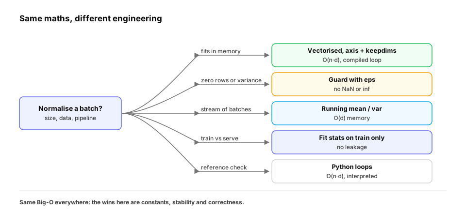
| If the constraint becomes… | Best approach | Time | Extra space |
|---|---|---|---|
| Teaching or reference check | Python loops, norm once per row | O(n·d), slow constant | O(n·d) output |
| Batch fits in memory | Vectorised NumPy, axis + keepdims |
O(n·d), fast constant | O(n) or O(d) stats |
| Zero rows / constant columns | Guard denominators with eps | same | same |
| Data doesn't fit in memory | Streaming mean / variance (Welford) | O(n·d) total | O(d) |
| Large offsets, float32 | Welford; never E[x²] − E[x]² |
O(n·d) | O(d) |
| Training vs serving | Fit stats on train, store, reuse | O(d) per value served | O(d) |
| Very large batches on GPU | Same maths in PyTorch / JAX | O(n·d), parallel | O(d) |
Quick check
Why compute variance with Welford's algorithm instead of E[x²] − E[x]² when streaming?
Show the answer
A. When values are large, E[x²] and E[x]² are huge and nearly equal, so their difference loses almost all precision to rounding; Welford updates deviations directly and stays accurate — Both are O(n·d) time and O(d) memory; the difference is numerical stability (catastrophic cancellation).
5. Saying it out loud
"Normalising is O(n·d) and that's optimal, since every value is read and written. The naive loop recomputes each norm per element, which makes it O(n·d²), so compute it once per row. Then vectorise:
X / norm(X, axis=1, keepdims=True), same complexity but compiled loops over a contiguous buffer. In production I'd guard zero norms and zero variances with an epsilon, stream statistics with Welford if the data doesn't fit, and fit the statistics on training data only."
Check yourself
- Why is the naive loop O(n · d²), and what fixes it?
- Why is the vectorised version faster if the complexity is the same?
- What does
keepdims=Truedo, and what goes wrong without it? - How do you avoid NaN for zero rows and constant columns?
- Why is
E[x²] − E[x]²dangerous, and what do you use instead? - Why fit normalisation statistics on the training set only?
Answers
- The norm (O(d)) is recomputed for each of the d elements in a row; compute it once per row.
- NumPy runs compiled loops over contiguous memory; Python pays interpreter overhead for every value. Same Big-O, much smaller constant.
- It keeps the reduced axis with size 1, e.g. norms of shape (n, 1), so broadcasting divides each row by its own norm; without it the shape is (n,), which broadcasts along columns instead.
- Divide by
max(norm, eps)and replace zero standard deviations (e.g. with 1) so constant columns become 0. - Catastrophic cancellation: both terms are huge and nearly equal. Use Welford's (or Chan's batched) update.
- Using test or serving data leaks information and makes outputs depend on the rest of the batch; stored training statistics give the same transform everywhere.