"What's the complexity?" is asked after every interview solution. Most candidates answer with a symbol they remember. Strong candidates derive it, out loud, from what the code does. This lesson builds Big-O from scratch: what we count, why we throw parts of the count away, how to read complexity straight from code, and how a constraint on the input changes which complexity is good enough.
The running example is range-sum queries, a pattern that shows up constantly in ML work (rolling windows over metrics, cumulative counts over time series). We'll take it from a brute force to an optimal solution, and see the exact moment the constraints force the optimisation.
1. Count operations, don't time them
Timing code tells you how fast it ran on one machine, for one input size. That's not what we need to know. We need to know how the cost grows as the input grows, because that's what decides whether a solution survives n = 10⁶.
So we count basic steps (a comparison, an addition, an index lookup) as a function of n:
| Code | Steps for input size n |
|---|---|
| Sum a list | about n additions |
| Compare every pair | about n²/2 comparisons |
| Binary search a sorted list | about log₂ n comparisons |
The counts let us predict without running anything. If n grows 10×, a linear algorithm does 10× the work and a quadratic one does 100×.
def count_ops(n):
    """Count how often the innermost line runs for common code shapes."""
    single = sum(1 for _ in range(n))                                   # one loop
    pairs = sum(1 for i in range(n) for _ in range(i + 1, n))           # every pair i < j
    halvings, m = 0, n
    while m > 1:                                                        # halve until 1
        m //= 2
        halvings += 1
    return single, pairs, halvings


for n in (10, 100, 1000):
    single, pairs, halvings = count_ops(n)
    assert single == n
    assert pairs == n * (n - 1) // 2
    assert halvings == n.bit_length() - 1                               # floor(log2 n)
    print(f"n={n:>5}: loop={single:>6}  pairs={pairs:>7}  halvings={halvings}")
Notice: going from n = 100 to 1,000 multiplies loop by 10, pairs by about 100, and adds just 3 to halvings.
That growth pattern is what Big-O describes.
2. Why constants and small terms disappear
Suppose an algorithm does exactly 3n² + 50n + 200 steps. Which part matters?
| n | 3n² | 50n | 200 | share from 3n² |
|---|---|---|---|---|
| 10 | 300 | 500 | 200 | 30% |
| 1,000 | 3,000,000 | 50,000 | 200 | 98% |
| 1,000,000 | 3 × 10¹² | 5 × 10⁷ | 200 | 99.998% |
As n grows, the fastest-growing term takes over and the others become noise. The constant 3 doesn't change the shape either: double n and the cost still quadruples. So we write O(n²): "grows no faster than a constant times n², for large n".
Two caveats you should say in interviews:
- Constants do matter between algorithms of the same class (a tight O(n) loop vs one doing 50 operations per element). Big-O decides which class; benchmarking decides which implementation.
- Big-O usually means the worst case. Say which case you mean when it differs: hash lookups are O(1) on average, O(n) in the pathological worst case.
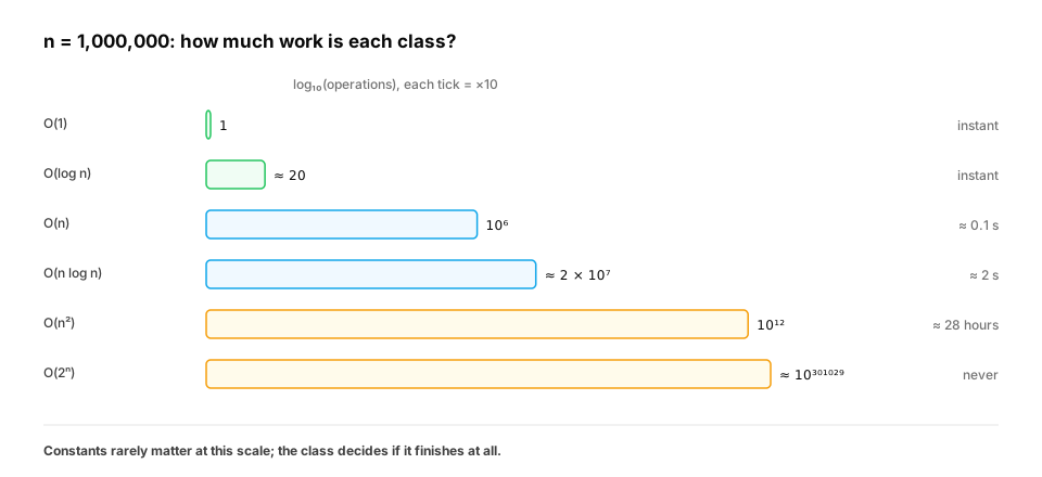
At n = 10⁶ the difference between classes isn't 2× or 10×. It's the difference between a tenth of a second and more than a day. That's why we classify first and micro-optimise later.
3. Reading complexity from the shape of code
You rarely need algebra. Look at the shape:
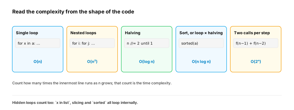
| Shape | Why | Complexity |
|---|---|---|
| One loop over the input | body runs n times | O(n) |
| A loop inside a loop | n × n | O(n²) |
| Halve the problem each step | after k steps n/2ᵏ = 1 → k = log₂ n | O(log n) |
| n items, each doing a halving, or a good sort | n × log n | O(n log n) |
| Each call makes two calls on size n − 1 | the call tree doubles per level | O(2ⁿ) |
| Two inputs of sizes n and m | depends on how they're combined | O(n + m) or O(n · m) |
The one rule: find the line that runs the most, and count how many times it runs as a function of the input sizes.
Hidden loops
Some single lines are loops in disguise. These are the most common way an "O(n)" solution is really O(n²):
| Looks like one step | Actually | Cost |
|---|---|---|
x in some_list |
scans the list | O(n) |
some_list.index(x), .count(x), .remove(x) |
scans the list | O(n) |
a[i:j] |
copies j − i items | O(j − i) |
s = s + piece in a loop |
builds a new string each time | O(total length) per step |
sorted(a) |
sorts | O(n log n) |
list.insert(0, x), list.pop(0) |
shifts every item | O(n) |
A real example. Removing duplicates while keeping order, written naturally:
import random
import time


def dedupe_slow(items):
    out = []
    for x in items:
        if x not in out:          # hidden loop: scans `out` every time
            out.append(x)
    return out


def dedupe_fast(items):
    seen, out = set(), []
    for x in items:
        if x not in seen:         # O(1) average: a set, not a list
            seen.add(x)
            out.append(x)
    return out


items = [random.randint(0, 4000) for _ in range(8000)]
assert dedupe_slow(items) == dedupe_fast(items)

t0 = time.perf_counter(); dedupe_slow(items); slow = time.perf_counter() - t0
t0 = time.perf_counter(); dedupe_fast(items); fast = time.perf_counter() - t0
print(f"slow {slow * 1000:.1f} ms, fast {fast * 1000:.2f} ms")
assert fast < slow
Same output, same-looking code. The slow version is O(n²) because x not in out scans a list that grows to n;
the fast one is O(n) because a set answers membership in O(1) on average. Changing one data structure changed
the class.
Quick check
Which line turns this loop into O(n²)? for x in a: if x not in b_list: c.append(x)
Show the answer
B. x not in b_list, because list membership scans the whole list each time — Membership tests on a list are linear scans. Inside a loop they multiply, giving O(n · m).
4. A full walkthrough: range-sum queries
Problem. You're given an array a of n numbers and q queries. Each query (l, r) asks for
a[l] + a[l+1] + … + a[r]. Return all answers.
ML context. A training dashboard asks "total loss between step 2,000 and step 3,000" for many ranges; a feature pipeline computes "clicks in the last k hours" for every user and every hour.
Step 1: Clarify
- Sizes: n up to 10⁵, q up to 10⁵.
- Values may be negative. Indices are 0-based and inclusive.
- Does the array change between queries? Assume no for now. (We'll change this later.)
Step 2: Brute force
Answer each query by adding up its range.
def range_sums_brute(a, queries):
    answers = []
    for l, r in queries:
        total = 0
        for i in range(l, r + 1):       # up to n additions per query
            total += a[i]
        answers.append(total)
    return answers


a = [3, 1, 4, 1, 5, 9]
assert range_sums_brute(a, [(1, 3), (0, 5), (4, 4)]) == [6, 23, 5]
print("brute force works")
- Time: each query can cover the whole array, so worst case O(n · q).
- Space: O(1) beyond the output.
Check against the constraints: n · q = 10⁵ × 10⁵ = 10¹⁰ additions. At roughly 10⁷ per second, that's about 17 minutes. Too slow, so we must optimise. If q were 1, the brute force would be perfectly fine: the constraint on q is what forces the change.
Step 3: Optimise: what work is repeated?
Two overlapping queries, say (1, 1000) and (2, 1001), add up almost the same 999 numbers twice. Across 10⁵ queries we re-add the same values over and over.
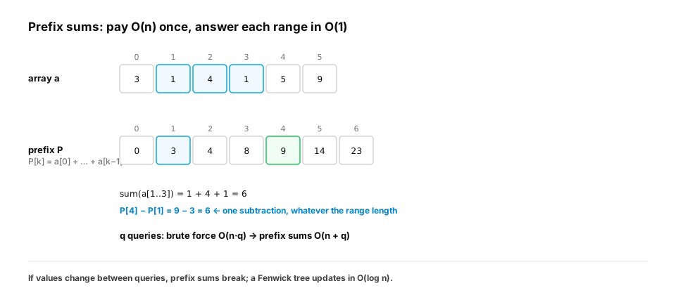
The first-principles fix: compute the running totals once, then reuse them. Define P[k] as the sum of the first
k values (P[0] = 0). Then any range is a difference of two running totals:
a[l] + … + a[r] = P[r + 1] − P[l]
from itertools import accumulate


def range_sums_prefix(a, queries):
    prefix = [0, *accumulate(a)]           # prefix[k] = a[0] + ... + a[k-1]; O(n) once
    return [prefix[r + 1] - prefix[l] for l, r in queries]   # O(1) per query


a = [3, 1, 4, 1, 5, 9]
assert range_sums_prefix(a, [(1, 3), (0, 5), (4, 4)]) == [6, 23, 5]
print("prefix sums work")
- Time: O(n) to build the prefix array, then O(1) per query: O(n + q). That's 2 × 10⁵ steps: instant.
- Space: O(n) for the prefix array. We traded memory for time, again.
Step 4 and 5: Code and test
Cross-check the fast version against the brute force on random inputs, including negative values and single-element ranges:
import random
from itertools import accumulate


def range_sums_brute(a, queries):
    return [sum(a[l:r + 1]) for l, r in queries]


def range_sums_prefix(a, queries):
    prefix = [0, *accumulate(a)]
    return [prefix[r + 1] - prefix[l] for l, r in queries]


rng = random.Random(1)
for _ in range(200):
    n = rng.randint(1, 30)
    a = [rng.randint(-50, 50) for _ in range(n)]
    queries = []
    for _ in range(rng.randint(1, 20)):
        l = rng.randrange(n)
        r = rng.randrange(l, n)
        queries.append((l, r))
    assert range_sums_prefix(a, queries) == range_sums_brute(a, queries)
print("prefix sums agree with brute force")
Step 6: Complexity, and what if the constraints change?
| If the constraint becomes… | Best approach | Time | Space |
|---|---|---|---|
| q = 1 (one query) | Brute force | O(n) | O(1) |
| Many queries, array fixed | Prefix sums | O(n + q) | O(n) |
| Values change between queries | Fenwick tree (binary indexed tree) | O(log n) per update and per query | O(n) |
| 2-D grid of values, rectangle queries | 2-D prefix sums | O(n·m + q) | O(n·m) |
| Queries arrive in a stream over a sliding window | Running window sum (module 04) | O(1) per step | O(1) |
The updates row matters: if a[i] changes, every P[k] with k > i changes too, so updating prefix sums costs
O(n). With many updates, that's back to O(n · q). A Fenwick tree keeps both operations at O(log n). You don't need it
yet; you need to notice that a new constraint breaks your current optimisation.
Quick check
With prefix sums built, the interviewer adds: 'between queries, single values can change'. What happens to your solution?
Show the answer
D. Each update invalidates up to n prefix values, so updates cost O(n) and the total can return to O(n · q); a structure like a Fenwick tree keeps updates and queries at O(log n) — Precomputation is only cheap while the data it summarises stays still. A new constraint (updates) breaks the trade.
5. Amortised cost: why append is O(1)
A Python list keeps spare capacity. Most appends just write into a free slot. When the list is full, Python
allocates a bigger block and copies everything: an O(n) step. So is append O(n)?
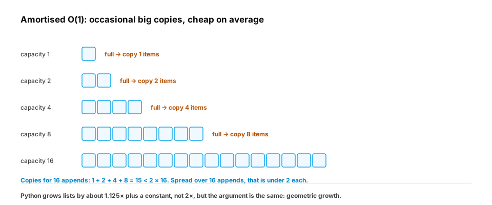
Add up the copies over n appends. With geometric growth, the copy sizes form a series like 1 + 2 + 4 + … which sums to less than 2n. Spread over n appends, that's fewer than 2 copies per append on average: amortised O(1). (CPython grows by about 1.125× rather than 2×; the series still sums to a constant times n.)
import sys

lst, resizes, last = [], 0, sys.getsizeof([])
for i in range(100_000):
    lst.append(i)
    size = sys.getsizeof(lst)
    if size != last:              # the underlying block was reallocated
        resizes += 1
        last = size
print(f"100,000 appends caused only {resizes} reallocations")
assert resizes < 200
"Amortised" is a promise about the total, not each call: one append can be slow, but any sequence of n appends
costs O(n).
6. Logarithms: the cost of halving
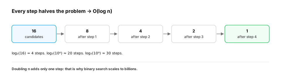
When each step halves what's left, the number of steps is how many times you can halve n before reaching 1: log₂ n.
| n | log₂ n |
|---|---|
| 1,000 | ≈ 10 |
| 1,000,000 | ≈ 20 |
| 1,000,000,000 | ≈ 30 |
Doubling n adds one step. That's why binary search (module 05) can search a billion sorted items in about 30 comparisons, and why O(n log n) sorting is only about 20× more work than reading the input once at n = 10⁶.
7. Two variables, and other traps
- Name your variables. "O(n)" is ambiguous when there are two inputs. Merging sorted lists of sizes n and m is O(n + m); comparing every element of one against the other is O(n · m). If m is tiny, O(n · m) may be fine.
- Output size counts. Returning all pairs of n items is at least O(n²) because the output has n² entries; no algorithm can beat writing its own answer.
- Recursion has a hidden cost. Each call uses stack space; a recursion of depth n is O(n) space even with no data structures (lesson 0.4).
- Average versus worst. Quickselect is O(n) average and O(n²) worst; hash tables O(1) average, O(n) worst. Say which you mean.
Quick check
Two sorted lists have sizes n and m. A two-pointer merge reads each element once. What is its time complexity?
Show the answer
C. O(n + m) — Each step advances one pointer, so the total number of steps is at most n + m.
8. Saying it out loud
"Brute force adds each range directly: O(n · q), 10¹⁰ here, too slow. The repeated work is re-adding overlapping ranges, so I'll precompute running totals once in O(n), and answer each query as a difference of two of them in O(1): O(n + q) time, O(n) extra space. If values could change between queries, prefix sums would need O(n) per update, so I'd switch to a Fenwick tree at O(log n) each."
Quick check
An algorithm runs in exactly 5n log₂ n + 1000n + 10⁶ steps. What is its Big-O, and why?
Show the answer
A. O(n log n), because for large n the n log n term grows fastest and the constants and smaller terms stop mattering — Big-O keeps the fastest-growing term and drops constants; n log n eventually dominates both n and the constant.
Check yourself
- Why count operations instead of measuring time?
- Why does
3n² + 50n + 200become O(n²)? When do constants still matter? - Name three single lines of Python that hide a loop.
- Walk through range-sum queries from brute force to prefix sums, with the constraint that forces the change.
- Why is
list.appendO(1) amortised even though a resize copies everything? - Why does doubling n add only one step to binary search?
Answers
- Time depends on the machine and one input size; operation counts show how cost grows with n, which decides feasibility.
- For large n, 3n² dominates the other terms, and the constant 3 doesn't change the growth shape. Constants matter when comparing two algorithms in the same class.
x in some_list,some_list.remove(x), slicinga[i:j],list.insert(0, x),sorted(a).- Brute force sums each range, O(n · q) = 10¹⁰ at the limits, too slow. Overlapping ranges repeat additions, so build
prefix sums once in O(n) and answer each query as
P[r+1] − P[l]in O(1): O(n + q). - Capacity grows geometrically, so total copying over n appends is under a constant times n: O(1) per append on average.
- Each comparison halves the remaining range, so the number of steps is log₂ n, and log₂(2n) = log₂ n + 1.