Arrays are the data structure ML runs on. A batch of images is a 4-D array; a sequence of token embeddings is a 2-D array; a time series of losses is a 1-D array. Interview problems on arrays look simple, but the strong answers come from understanding how an array is laid out in memory, because that layout explains which operations are free, which copy everything, and why "vectorised" code is fast.
This lesson builds that model from first principles: memory layout, index arithmetic for multi-dimensional data, copies versus views, batching, and then one complete problem, rolling-window averages over a time series, solved three ways as the constraints change.
1. An array is a start address plus index arithmetic
An array stores elements next to each other. If element 0 lives at address start and each element takes s
bytes, element i lives at start + i × s. Finding it is one multiply and one add: that's why indexing is O(1),
no matter how long the array is.
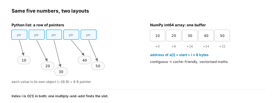
Python gives you two kinds:
Python list |
NumPy array (int64, float32, …) |
|
|---|---|---|
| Stores | pointers to separate objects | raw values in one buffer |
| Bytes per number | ≈ 36 (pointer + int object) | 8 (or 4, 2, 1 by dtype) |
| Element types | anything, mixed | one fixed type |
| Indexing | O(1) | O(1) |
| Whole-array maths | a Python loop: slow | one compiled loop: fast |
The list's flexibility (any object, any mix) costs memory and speed. NumPy's restriction (one type, packed) buys compactness and lets a single compiled loop process millions of values: vectorisation.
2. Multi-dimensional arrays are flat arrays plus arithmetic
A 3 × 4 matrix isn't stored as a grid. It's stored as 12 values in a row, row after row (row-major, the
default in NumPy and C). Element (i, j) lives at flat index i × cols + j.
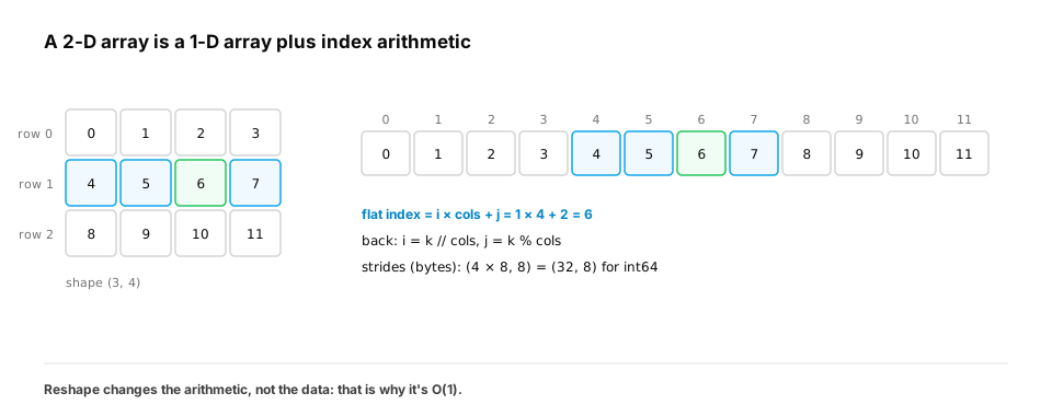
This one idea explains a lot of tensor behaviour:
- Shape
(3, 4)says how to interpret the flat buffer. - Strides say how many bytes to jump for one step along each axis:
(4 × 8, 8)for int64. Moving down a row jumps 32 bytes; moving right jumps 8. - Reshape to
(4, 3)or(12,)changes only shape and strides: O(1), no data moves. - Transpose swaps strides: also O(1) in NumPy, but the result is no longer row-contiguous, so some later operations copy it.
import numpy as np


def flat_index(i, j, cols):
    return i * cols + j


def unflat(k, cols):
    return k // cols, k % cols


rows, cols = 3, 4
grid = np.arange(rows * cols).reshape(rows, cols)          # values 0..11, row-major
flat = grid.ravel()

for i in range(rows):
    for j in range(cols):
        k = flat_index(i, j, cols)
        assert flat[k] == grid[i, j]
        assert unflat(k, cols) == (i, j)

assert grid.strides == (cols * grid.itemsize, grid.itemsize)   # (32, 8) for int64
assert np.shares_memory(grid, grid.reshape(cols, rows))         # reshape: same buffer, no copy
print("flat index of (1, 2):", flat_index(1, 2, cols), "strides:", grid.strides)
In interviews: "rotate a matrix", "spiral order", "set matrix zeroes" (later in this module) are all exercises in
this index arithmetic. Think in (i, j) → i × cols + j and the bugs disappear.
Quick check
Why is reshaping a NumPy array from (1000, 768) to (768000,) O(1)?
Show the answer
B. Reshape only changes the shape and strides that interpret the same contiguous buffer; no element is moved — A contiguous array's layout already matches the new shape, so only the metadata changes.
3. Slices: copies or views?
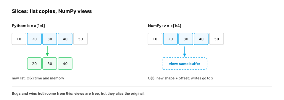
This is where many subtle bugs (and many free speed-ups) come from.
list[a:b] |
NumPy x[a:b] |
|
|---|---|---|
| What you get | a new list | a view (same buffer) |
| Cost | O(b − a) time and memory | O(1) |
| Writing to it | doesn't affect the original | changes the original |
import numpy as np

# Python list: slicing copies.
a = [10, 20, 30, 40, 50]
b = a[1:4]
b[0] = 999
assert a == [10, 20, 30, 40, 50]                 # original untouched

# NumPy: basic slicing is a view.
x = np.array([10, 20, 30, 40, 50])
v = x[1:4]
v[0] = 999
assert x.tolist() == [10, 999, 30, 40, 50]       # original changed through the view
assert np.shares_memory(x, v)

# Fancy indexing (a list of indices or a boolean mask) always copies.
c = x[[1, 2, 3]]
assert not np.shares_memory(x, c)
print("list slices copy; NumPy basic slices are views; fancy indexing copies")
Interview habit: when you write nums[1:] inside a loop or recursion, say "this slice copies, O(n) each time"
and pass indices (start, end) instead when it matters.
4. Batching: the most common array operation in ML
Problem. Split a dataset of n items into batches of size b. The last batch may be smaller; optionally drop it.
def batches(items, size, drop_last=False):
    for start in range(0, len(items), size):
        batch = items[start:start + size]             # one O(size) slice per batch
        if drop_last and len(batch) < size:
            return
        yield batch


data = list(range(10))
assert list(batches(data, 4)) == [[0, 1, 2, 3], [4, 5, 6, 7], [8, 9]]
assert list(batches(data, 4, drop_last=True)) == [[0, 1, 2, 3], [4, 5, 6, 7]]
assert list(batches([], 4)) == []
print("batching works: O(n) total, one batch in memory at a time")
- Time: O(n) total: every item is copied into exactly one batch.
- Space: O(b) at a time, because it's a generator (lesson 0.4): only the current batch exists.
- With NumPy,
x[start:start + b]would be a view: O(1) per batch and no copying at all.
5. A full problem: rolling averages over a time series
Problem. Given n values (say, training loss per step) and a window size k, return the mean of every window of k consecutive values. There are n − k + 1 windows.
values = [4, 8, 6, 2, 10, 4], k = 3 → [6.0, 5.33, 6.0, 5.33]
ML context. Smoothing a noisy loss curve, computing rolling features over sensor readings, moving averages of click rates.
Step 1: Clarify
- n up to 10⁶ steps; k anywhere from 2 to n.
- Return floats; if k > n, return an empty list.
- Memory: avoid materialising all windows if n and k are both large.
Step 2: Brute force: sum each window
def rolling_mean_brute(values, k):
    n = len(values)
    return [sum(values[i:i + k]) / k for i in range(n - k + 1)]   # each window: O(k) slice + O(k) sum


assert rolling_mean_brute([4, 8, 6, 2, 10, 4], 3) == [6.0, 16 / 3, 6.0, 16 / 3]
assert rolling_mean_brute([1, 2], 3) == []
print("brute force works")
- Time: (n − k + 1) windows × O(k) each = O(n · k). With n = 10⁶ and k = 1,000 that's about 10⁹ additions: minutes in Python.
- Space: O(k) for each slice, plus the output.
Against the constraints: when k is large the brute force is too slow, and the constraint that bites is k, not n. With k = 3, the brute force is fine.
Step 3: Optimise: what work is repeated?
Two neighbouring windows share k − 1 values. Moving one step right, the window loses one value on the left and gains one on the right. So update the sum instead of recomputing it:
sum(window i+1) = sum(window i) − values[i] + values[i + k]
def rolling_mean_running(values, k):
    n = len(values)
    if k > n:
        return []
    window = sum(values[:k])                    # the first window, O(k) once
    out = [window / k]
    for i in range(k, n):
        window += values[i] - values[i - k]     # add the newcomer, drop the leaver: O(1)
        out.append(window / k)
    return out


import random

rng = random.Random(0)
for _ in range(300):
    n = rng.randint(0, 40)
    values = [rng.randint(-50, 50) for _ in range(n)]
    k = rng.randint(1, 45)
    fast, slow = rolling_mean_running(values, k), [sum(values[i:i + k]) / k for i in range(n - k + 1)]
    assert len(fast) == len(slow) and all(abs(a - b) < 1e-9 for a, b in zip(fast, slow))
print("running sum matches brute force: O(n) instead of O(n·k)")
- Time: O(k) for the first window, then O(1) per step: O(n), whatever k is.
- Space: O(1) beyond the output.
- This is the sliding window pattern, which gets its own module (04).
Step 4: When the constraints change: vectorise with prefix sums
In Python, even O(n) means a million interpreted loop steps (a fraction of a second). If this runs inside a data pipeline over thousands of series, the constant factor matters. Prefix sums (lesson 1.2) give every window sum at once as a difference of two cumulative sums, and NumPy does it in compiled code:
import numpy as np


def rolling_mean_numpy(values, k):
    x = np.asarray(values, dtype=np.float64)
    if k > len(x):
        return np.array([])
    c = np.concatenate(([0.0], np.cumsum(x)))       # prefix sums, O(n), vectorised
    return (c[k:] - c[:-k]) / k                      # every window at once


def rolling_mean_view(values, k):
    x = np.asarray(values, dtype=np.float64)
    windows = np.lib.stride_tricks.sliding_window_view(x, k)   # (n-k+1, k) VIEW, no copy
    assert np.shares_memory(windows, x)
    return windows.mean(axis=1)                                  # still O(n·k) arithmetic


values = [4, 8, 6, 2, 10, 4]
assert np.allclose(rolling_mean_numpy(values, 3), [6, 16 / 3, 6, 16 / 3])
assert np.allclose(rolling_mean_view(values, 3), rolling_mean_numpy(values, 3))

big = np.random.default_rng(1).normal(size=200_000)
assert np.allclose(rolling_mean_numpy(big, 500), rolling_mean_view(big, 500))
print("vectorised versions agree")
Note the trap in rolling_mean_view: the windows are a free view, but mean(axis=1) still does n · k additions.
A view saves memory, not arithmetic. The prefix-sum version does O(n) arithmetic.
Step 5: Complexity, and how the answer changes
| If the constraint becomes… | Best approach | Time | Extra space |
|---|---|---|---|
| k tiny (≤ 5), n small | Brute force slices | O(n · k) | O(k) |
| Any k, plain Python | Running sum | O(n) | O(1) |
| Many long series, speed matters | NumPy prefix sums | O(n), vectorised | O(n) |
| Need every window's values (not just means) | sliding_window_view |
O(1) to create | O(1) (a view) |
| Values arrive as a stream | Running sum + a queue of the last k | O(1) per value | O(k) |
| Rolling max instead of mean | Monotonic deque (module 06) | O(n) | O(k) |
The last row matters: the running-sum trick works because a sum can be un-added. A maximum can't be "un-maxed" when the largest value leaves the window, so a different structure is needed. Knowing why an optimisation works tells you when it stops working.
Quick check
Why can a rolling sum be updated in O(1) per step, but a rolling maximum can't be updated the same way?
Show the answer
C. Subtraction undoes addition, so the leaving value can be removed from the sum; there's no operation that removes the leaving value from a maximum if it was the maximum — Incremental updates need an inverse operation. Sums have one; max doesn't, so it needs a different structure.
6. Saying it out loud
"Brute force slices and sums every window: O(n · k), up to 10⁹ here. Neighbouring windows share k − 1 values, so I keep a running sum, add the value entering and subtract the one leaving: O(n) time, O(1) space. If this ran over many series I'd vectorise with NumPy prefix sums: window sums are differences of cumulative sums. If they asked for a rolling max instead, the subtraction trick fails because max has no inverse, so I'd use a monotonic deque."
Quick check
A function receives a NumPy array x and does y = x[100:200]; y *= 2. The caller is surprised that x changed. Why, and what fixes it?
Show the answer
A. Basic slicing returns a view sharing x's buffer, so in-place multiplication writes into x; use x[100:200].copy() (or a non-in-place y = y * 2) when you need independence — Views make slicing free but alias the original. Copy explicitly when you intend to modify independently.
Check yourself
- Why is
a[i]O(1) for both Python lists and NumPy arrays? - Where is element (i, j) of a row-major R × C array in the flat buffer, and how do you invert it?
- What does a list slice cost, and how does a NumPy basic slice differ?
- Take rolling averages from brute force to a running sum to NumPy prefix sums, with the constraint that justifies each.
- Why does
sliding_window_view(...).mean(axis=1)still cost O(n · k)? - Why doesn't the running-sum trick work for a rolling maximum?
Answers
- Elements are at evenly spaced addresses (pointers for lists, raw values for NumPy), so slot i's address is computed directly.
- At
i × C + j; invert withi = k // C,j = k % C. - A list slice copies: O(length) time and memory. A NumPy basic slice is a view: O(1), sharing (and aliasing) the buffer.
- Brute force O(n·k) is fine for tiny k; a running sum gives O(n) for any k; NumPy prefix sums keep O(n) but run in compiled code when there are many long series.
- The view avoids copying windows, but the mean still adds k values for each of the n − k + 1 windows.
- A sum can subtract the value leaving the window; a max can't "remove" the leaving value if it was the maximum.